flowchart LR
    A[Business Question] --> B[Fit Regression Model]
    B --> C[Check Assumptions Post Hoc]
    C --> D[Decide Whether the Model Is Trustworthy]
Part 2B: Regression Assumptions — What They Mean, Why They Matter, and How to Check Them
ImportantThe goal of this section
Linear regression can be very useful, but only if we understand when the model is behaving reasonably well.
This section explains four core assumptions often discussed in an introductory regression course:
- Linearity
- Normal residuals
- Constant variance
- Uncorrelated residuals
For each one, we will cover:
- what the assumption means,
- why it matters,
- what graphs and outputs to examine,
- and how to interpret what you see.
1. Why Regression Assumptions Matter
A regression model is a simplified description of reality.
That is not a flaw. It is the whole point of modeling. We use a simpler structure to help us understand patterns and support decisions.
But if the model is too far from the way the data actually behave, then:
- coefficients may be misleading,
- standard errors may be unreliable,
- p-values may be less trustworthy,
- confidence intervals may be inaccurate,
- and predictions may be worse than they appear.
Note
Regression assumptions are not mainly about making a model “perfect.” They are about helping us decide whether the model is good enough to trust for interpretation and decision-making.
1.1 Assumption Checking Is a Post Hoc Process
In most regression workflows, assumption checking happens after a model has been fit.
That is why it is often called a post hoc diagnostic process.
The usual sequence is:
- Start with a business question
- Fit a regression model
- Examine residuals and diagnostic plots
- Decide whether the model seems reasonable enough to interpret
This is important because assumptions are rarely something we can fully verify before fitting the model. We usually need the fitted line and the residuals before we can diagnose how well the model is behaving.
ImportantPractical takeaway
Assumption checking is usually not something you do before regression. It is something you do after fitting the model, by looking at the residuals and the structure of the problem.
2. A Useful Big Picture
You can think of regression diagnostics as asking four questions:
- Linearity: Is a straight line a reasonable summary of the relationship?
- Normal residuals: Are the residuals distributed in a way that makes our inference procedures work reasonably well?
- Constant variance: Is the amount of scatter around the line about the same across the range of fitted values?
- Uncorrelated residuals: Are the residuals independent from one observation to the next, or is there a pattern of dependence?
flowchart LR
    A[Fit Regression Model] --> B[Check Residual Plots]
    B --> C[Check Distribution of Residuals]
    C --> D[Check Dependence Structure]
    D --> E[Decide Whether Model Is Reasonable]
3. What Residuals Are
Before checking assumptions, students need a clear idea of what a residual is.
A residual is the part of an observation that the regression line does not explain.
It is calculated as:
\[ \text{Residual} = \text{Actual Value} - \text{Predicted Value} \]
or, using symbols:
\[ e_i = y_i - \hat{y}_i \]
where: - \(y_i\) is the actual observed value for observation \(i\), - \(\hat{y}_i\) is the predicted value from the regression line, - and \(e_i\) is the residual.
Example
Suppose for one observation:
- actual sales = 210
- predicted sales = 195
Then the residual is:
\[ 210 - 195 = 15 \]
That means the observation is 15 units above the fitted line.
If instead:
- actual sales = 180
- predicted sales = 195
then the residual is:
\[ 180 - 195 = -15 \]
That means the observation is 15 units below the fitted line.
Why residuals matter
Residuals are central to regression diagnostics because they tell us what the model failed to explain.
If the model is behaving reasonably well, the residuals should not show strong systematic structure.
Note
A lot of regression diagnostics can be summarized this way:
After fitting the line, do the leftover errors still show a pattern?
4. Set Up: Simulated Data for Diagnostics
We will simulate several small examples so you can see what different diagnostic patterns look like.
5. Assumption 1: Linearity
5.1 What linearity means
The linearity assumption means that the average relationship between \(X\) and \(Y\) can be reasonably summarized by a straight line.
That does not mean every point has to lie near a straight line. Real data always have noise.
It means that the overall mean structure is reasonably linear.
In simple linear regression, we are assuming that:
\[ E(Y \mid X) = \beta_0 + \beta_1 X \]
In plain language:
The expected value of \(Y\), given \(X\), changes in a straight-line way as \(X\) changes.
5.2 Why linearity matters
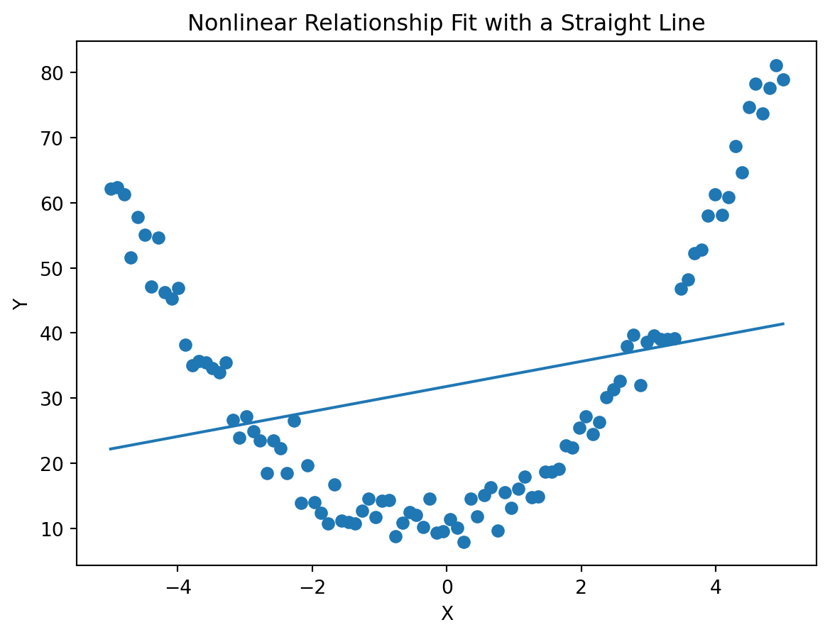
If the true relationship is strongly curved and we fit a straight line anyway, then:
- the slope may be misleading,
- predictions may be biased,
- and the fitted line may systematically miss important structure.
This matters because the regression line is supposed to summarize the average relationship. If the shape is wrong, the interpretation can be wrong.
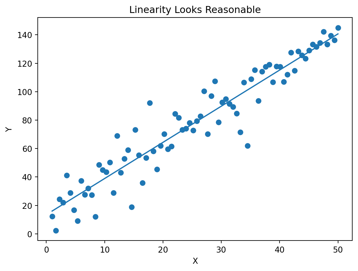
5.3 What to look for
The two most useful visuals are:
- the scatterplot with fitted line
- the residuals versus fitted values plot
If the model is reasonably linear, residuals should not show a strong curved pattern.
5.4 Example: Relationship is approximately linear
Residual view
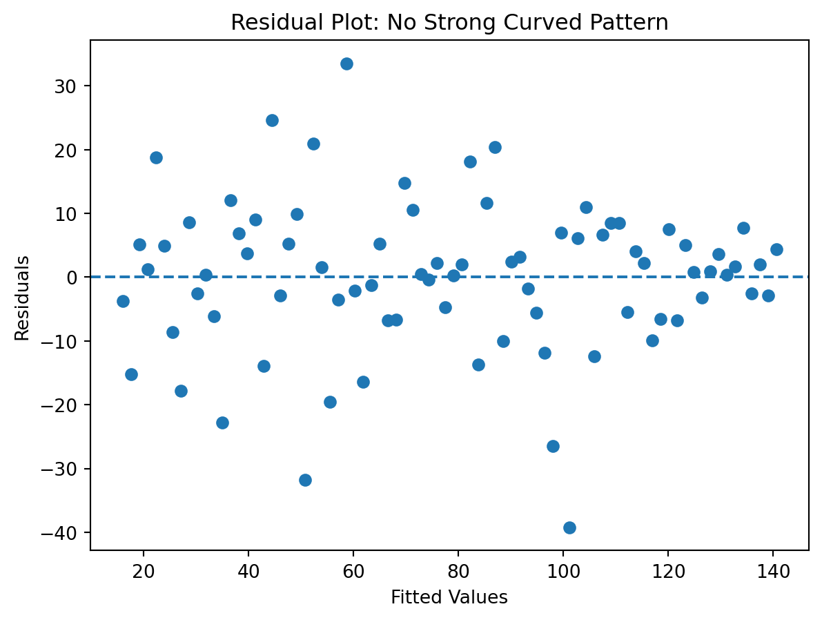
When linearity is reasonable, the residuals tend to look like a cloud around zero without strong systematic curvature.
5.5 Example: Relationship is nonlinear
Residual view
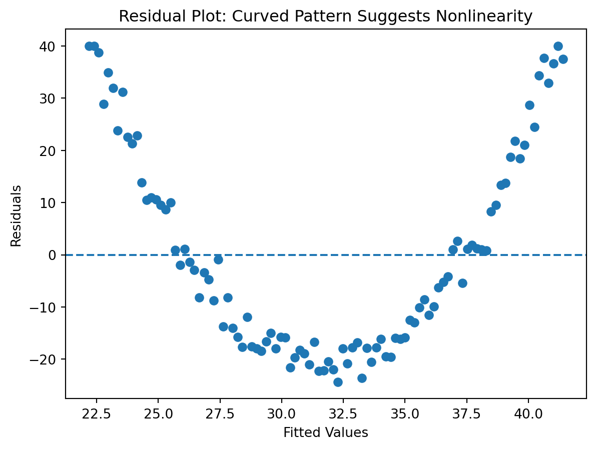
This is exactly what we do not want.
The residuals are not randomly scattered around zero. Instead, they show a pattern, which suggests the straight-line model is missing structure.
Warning
A curved residual pattern is one of the clearest signs that the linearity assumption may be violated.
6. Assumption 2: Normal Residuals
6.1 What normal residuals means
This assumption does not mean that \(X\) or \(Y\) must be normally distributed.
It refers to the residuals.
The idea is that the residuals are approximately normally distributed, especially if we want to rely on the usual t-tests, p-values, and confidence intervals in small to moderate samples.
A key detail is that the residual distribution should be centered around zero. That makes sense because residuals are the leftover errors after fitting the line. If the model is systematically overpredicting or underpredicting, the residuals would not be centered properly.
6.2 Why normal residuals matter
Normal residuals are mainly important for inference:
- hypothesis tests,
- p-values,
- confidence intervals.
They are less important for the basic idea of fitting a line.
If residuals are somewhat non-normal, the model may still be useful, especially in large samples. But if the residual distribution is highly skewed or has extreme outliers, then the standard inference can be less reliable.
6.3 What to look for
Common diagnostics include:
- a histogram of residuals
- a Q-Q plot
- signs of heavy skewness or extreme outliers
What you want to see
In a histogram of residuals, you usually hope to see: - the distribution centered near zero, - a roughly symmetric shape, - and no extreme strange tails or isolated spikes.
In a Q-Q plot, you usually hope to see: - points falling roughly along a straight reference line, - with only modest departures at the ends.
For MBA-level interpretation, the most important question is not:
“Is it perfectly normal?”
The more useful question is:
“Is it close enough to normal that the usual inference seems reasonable?”
6.4 Example: Residuals that are roughly normal
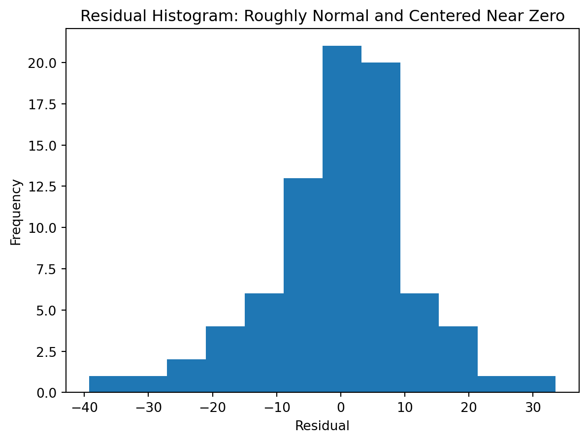
This is not perfect, but it is roughly bell-shaped and centered around zero. In many practical settings, this would be acceptable.
6.5 Example: Residuals that are clearly skewed
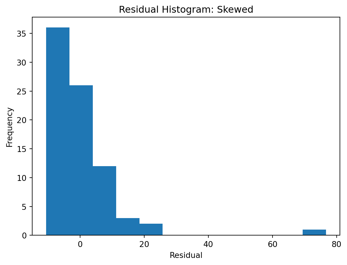
This residual distribution is clearly less symmetric. That does not automatically ruin the model, but it is a warning sign for inference.
Note
In large samples, regression is often fairly robust to moderate non-normality. In smaller samples, strong non-normality is more concerning.
7. Assumption 3: Constant Variance
7.1 What constant variance means
Constant variance means the spread of the residuals is roughly the same across the range of fitted values or across the range of \(X\).
This assumption is also called:
- homoscedasticity = constant variance
- heteroscedasticity = changing variance
7.2 Why constant variance matters
If variance changes substantially across the data, then:
- standard errors may be wrong,
- p-values may be misleading,
- confidence intervals may be too narrow or too wide,
- and other measures of uncertainty can be distorted.
So even if the fitted line still captures the average trend reasonably well, our uncertainty statements may become less trustworthy.
That means you could: - think a slope is significant when it is not, - fail to detect a real relationship, - or report misleading confidence intervals.
7.3 What to look for
The main diagnostic is:
- residuals versus fitted values
When constant variance holds reasonably well, the residual spread should look fairly even across the plot.
When it fails, you often see:
- a funnel shape,
- a megaphone shape,
- or visibly changing spread.
7.4 Example: Constant variance looks reasonable
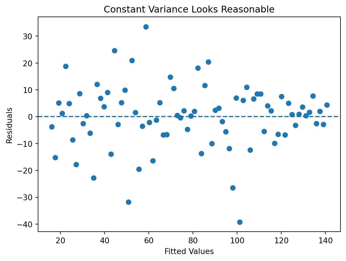
Here, the vertical spread is not perfectly identical everywhere, but it is fairly stable.
7.5 Example: Non-constant variance
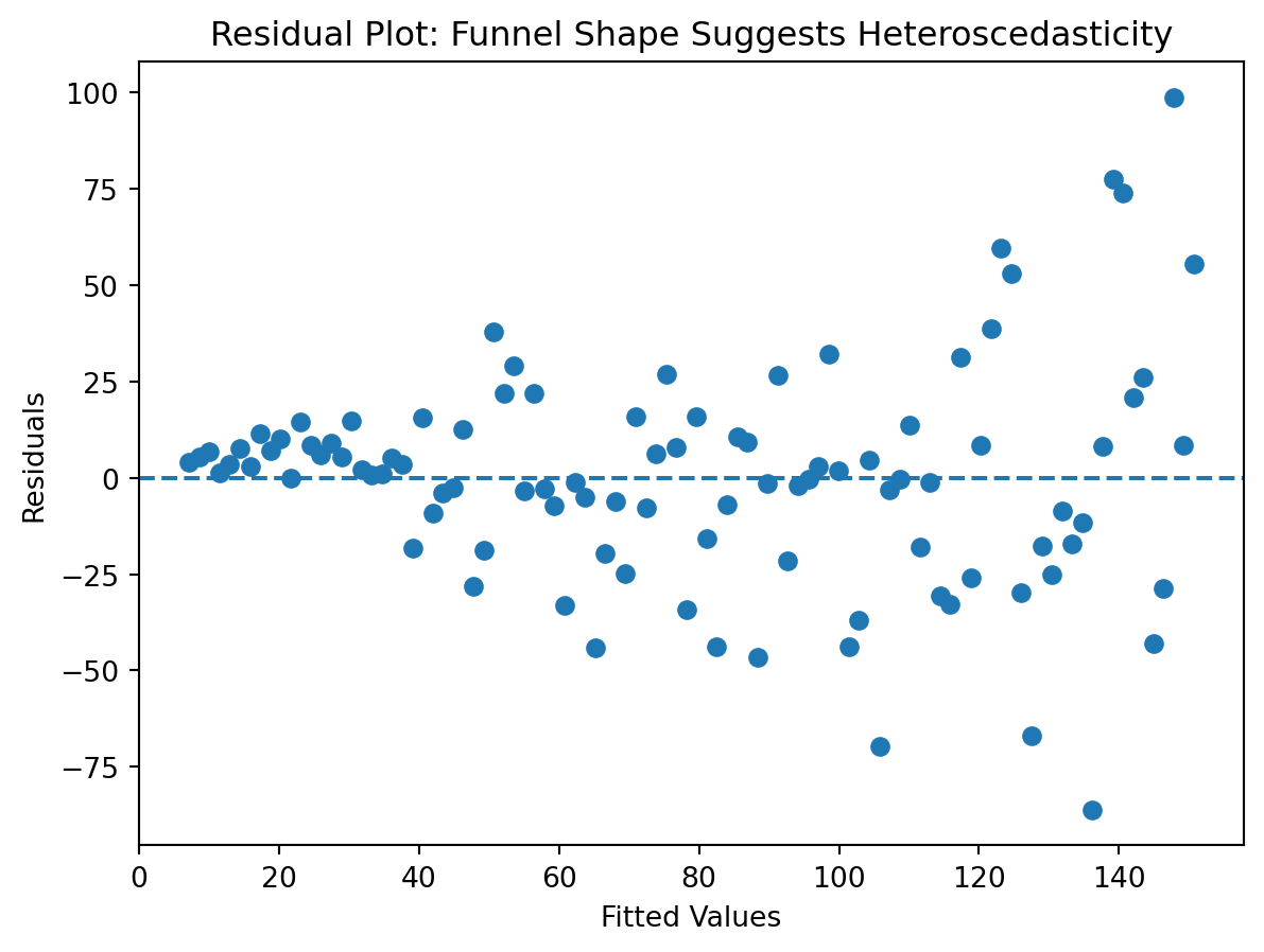
This funnel shape is one of the classic visual signs of non-constant variance.
Warning
If the residual spread grows or shrinks systematically, the constant variance assumption may not hold.
8.2 Why this matters
If residuals are correlated, then the model has usually missed some structure.
This often happens because of the problem structure, not because the analyst did something careless.
The most common situations are:
- time series data, where nearby observations are related over time,
- multiple measures on the same person, store, or company,
- repeated observations inside the same cluster or unit.
In those situations, independence is not mainly about a graph. It is about how the data were generated.
ImportantKey idea about independence
The independence or uncorrelated-residuals assumption is often best understood from the structure of the problem.
If your data come from time order, repeated measures, or clusters, dependence is often plausible before you ever make a plot.
8.3 What to look for
Useful clues include:
- knowing whether the data are time ordered,
- asking whether the same unit appears multiple times,
- plotting residuals in observation order or over time.
If residuals show long runs above zero and then below zero, that can suggest correlation.
8.4 Example: Residuals that are mostly uncorrelated
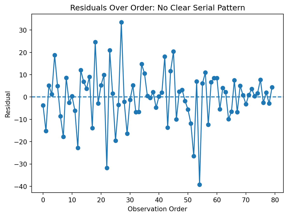
This looks fairly random over order. That is more consistent with uncorrelated residuals.
8.5 Example: Residuals that appear correlated over time
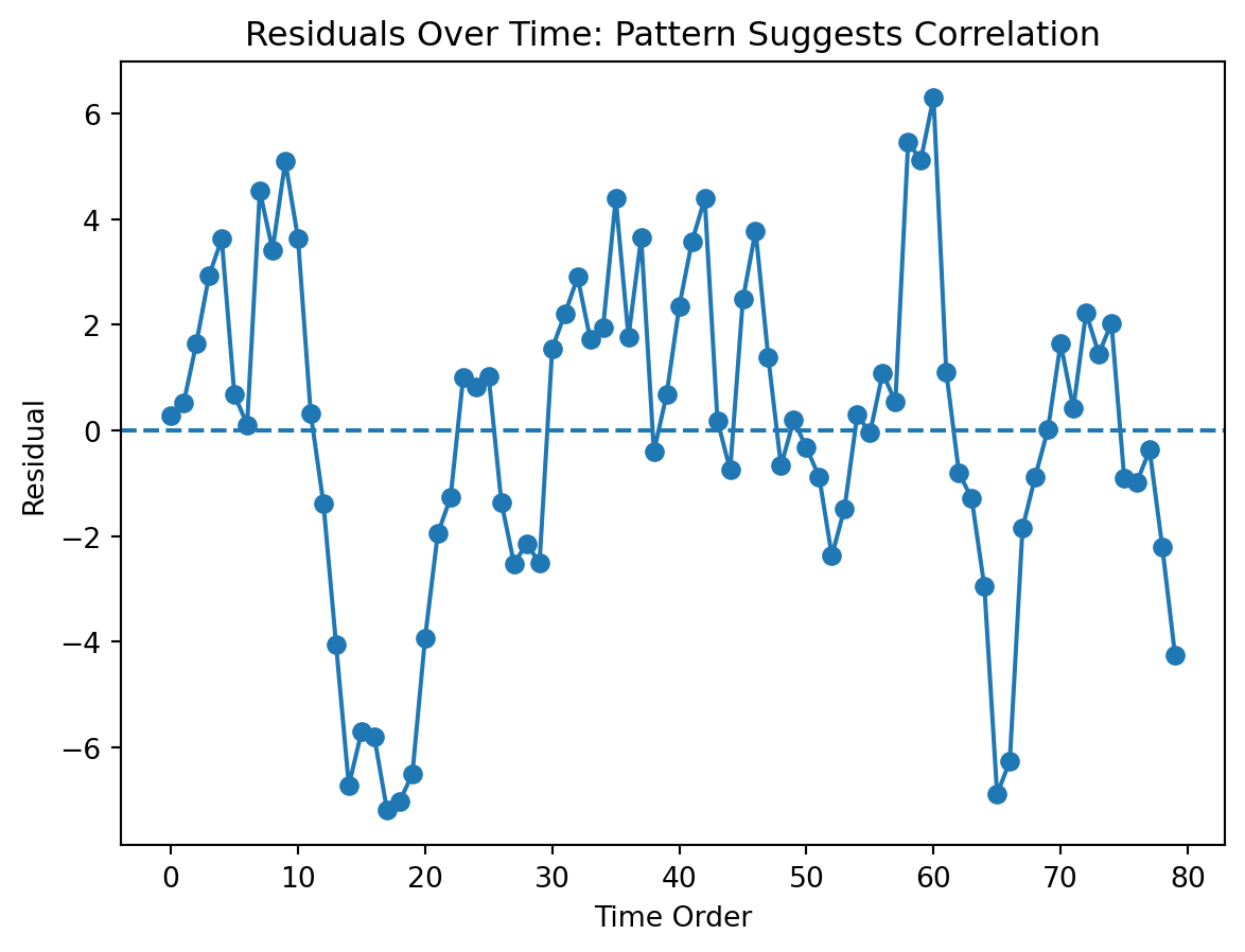
Notice how the residuals move in runs rather than bouncing randomly around zero.
That is often a clue that the errors are correlated over time.
8.6 Why independence is often about the data structure
This assumption deserves special emphasis because students often treat it like just another graph to inspect.
But in practice, you should ask first:
- Are these observations collected over time?
- Do I have multiple observations from the same person, customer, store, or region?
- Are there repeated measurements?
- Is there a natural ordering that could create persistence?
If the answer is yes, then correlated residuals become much more plausible.
Examples
- Monthly sales over time: nearby months may be similar
- Repeated employee evaluations: the same employee appears multiple times
- Store-level weekly data: nearby weeks in the same store may be correlated
- Patient follow-up visits: repeated observations on the same patient are not independent
In those settings, ordinary regression may still be a useful first pass, but the independence assumption is more questionable.
9. Putting the Assumptions Together
Here is a compact summary.
| Assumption | What it means | Why it matters | What to check |
|---|---|---|---|
| Linearity | Mean relationship is reasonably straight-line | Wrong shape can bias interpretation | Scatterplot, residuals vs fitted |
| Normal residuals | Residuals are roughly normal and centered near zero | Helps p-values and intervals work better | Histogram, Q-Q plot |
| Constant variance | Residual spread stays roughly stable | Standard errors, p-values, and uncertainty depend on it | Residuals vs fitted |
| Uncorrelated residuals | Residuals do not show dependence | Inference can be distorted if errors are related | Residuals over order/time, problem structure |
10. A Walkthrough of a Full Example Where Assumptions Mostly Hold
Let’s simulate a regression problem where the assumptions are mostly reasonable.
import numpy as np
import pandas as pd
import statsmodels.api as sm

np.random.seed(77)

x_demo = np.linspace(5, 60, 70)
y_demo = 18 + 2.4 * x_demo + np.random.normal(0, 10, len(x_demo))

df_demo = pd.DataFrame({"x": x_demo, "y": y_demo})

X_demo = sm.add_constant(df_demo["x"])
model_demo = sm.OLS(df_demo["y"], X_demo).fit()

print(model_demo.summary())
OLS Regression Results
==============================================================================
Dep. Variable: y R-squared: 0.948
Model: OLS Adj. R-squared: 0.947
Method: Least Squares F-statistic: 1242.
Date: Tue, 07 Apr 2026 Prob (F-statistic): 2.06e-45
Time: 16:03:33 Log-Likelihood: -256.48
No. Observations: 70 AIC: 517.0
Df Residuals: 68 BIC: 521.5
Df Model: 1
Covariance Type: nonrobust
==============================================================================
coef std err t P>|t| [0.025 0.975]
------------------------------------------------------------------------------
const 13.5241 2.578 5.245 0.000 8.379 18.669
x 2.5051 0.071 35.241 0.000 2.363 2.647
==============================================================================
Omnibus: 2.257 Durbin-Watson: 2.209
Prob(Omnibus): 0.323 Jarque-Bera (JB): 1.774
Skew: 0.387 Prob(JB): 0.412
Kurtosis: 3.096 Cond. No. 81.7
==============================================================================
Notes:
[1] Standard Errors assume that the covariance matrix of the errors is correctly specified.Scatterplot with fitted line
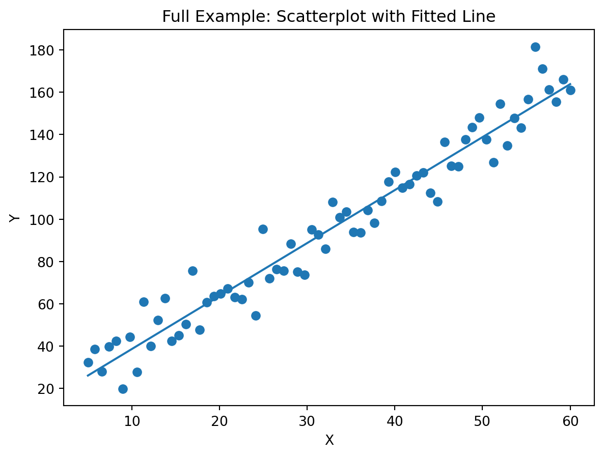
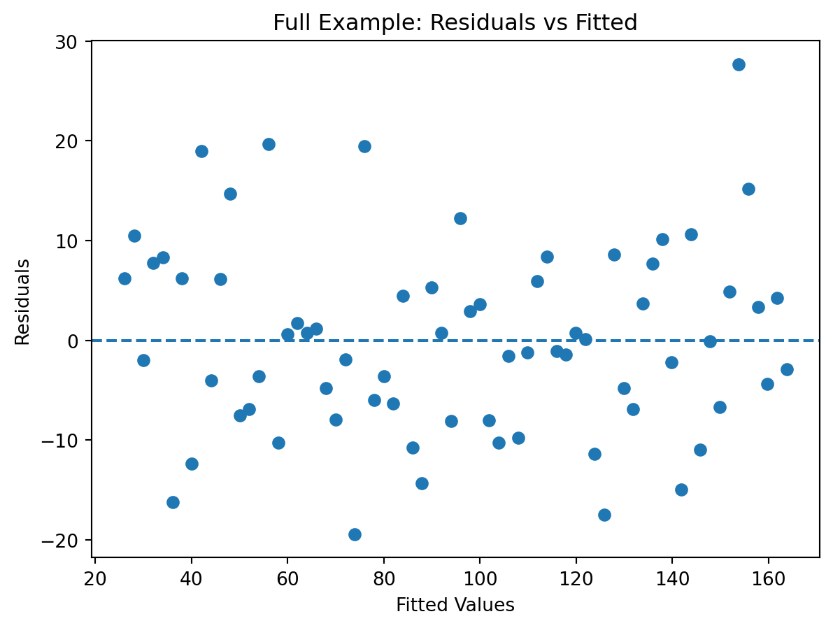
Residuals versus fitted
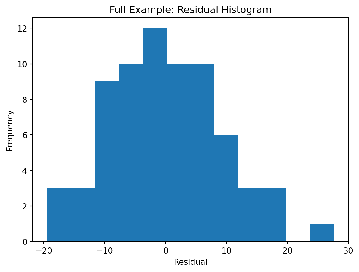
Histogram of residuals
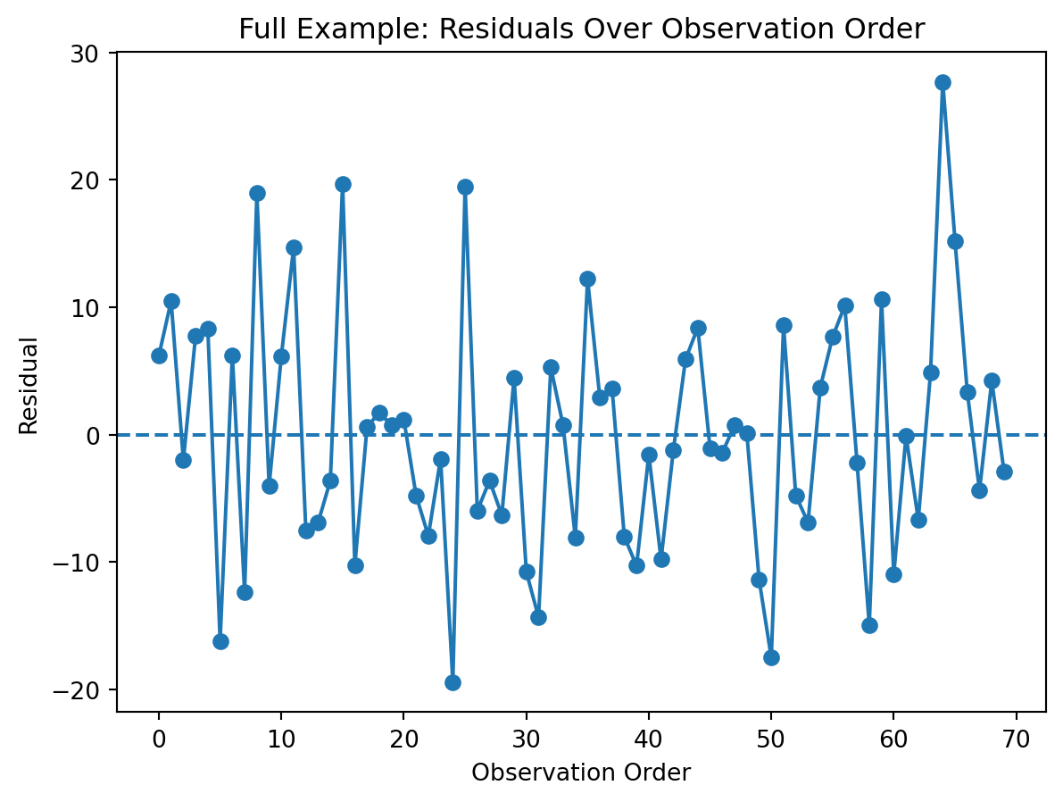
Residuals in observation order
How a student should read this example
A student should be able to say something like:
The scatterplot suggests that a straight-line relationship is reasonable. The residual plot does not show a strong curved pattern, so linearity seems acceptable. The spread of the residuals looks fairly stable, so constant variance seems reasonable. The histogram of residuals looks roughly symmetric and centered around zero, so normality does not appear to be a major concern. The residuals over order do not show an obvious run pattern, so uncorrelated residuals seems plausible here.
That is the kind of interpretation we want students to practice.
11. A Walkthrough of a Full Example Where Assumptions Are Violated
Now let’s create a more problematic example on purpose.
In this example, we build in: - a curved mean relationship, - changing residual spread, - and dependence over order.
np.random.seed(1234)

n_bad = 90
x_bad = np.linspace(1, 50, n_bad)

eps_bad = np.zeros(n_bad)
for t in range(1, n_bad):
    eps_bad[t] = 0.70 * eps_bad[t-1] + np.random.normal(0, 1 + 0.15 * x_bad[t])

y_bad = 12 + 1.2 * x_bad + 0.08 * (x_bad**2) + eps_bad

df_bad = pd.DataFrame({"x": x_bad, "y": y_bad})
X_bad = sm.add_constant(df_bad["x"])
model_bad = sm.OLS(df_bad["y"], X_bad).fit()

print(model_bad.summary())
OLS Regression Results
==============================================================================
Dep. Variable: y R-squared: 0.958
Model: OLS Adj. R-squared: 0.958
Method: Least Squares F-statistic: 2023.
Date: Tue, 07 Apr 2026 Prob (F-statistic): 1.64e-62
Time: 16:03:33 Log-Likelihood: -376.17
No. Observations: 90 AIC: 756.3
Df Residuals: 88 BIC: 761.3
Df Model: 1
Covariance Type: nonrobust
==============================================================================
coef std err t P>|t| [0.025 0.975]
------------------------------------------------------------------------------
const -23.4902 3.445 -6.818 0.000 -30.337 -16.643
x 5.3006 0.118 44.982 0.000 5.066 5.535
==============================================================================
Omnibus: 5.503 Durbin-Watson: 0.173
Prob(Omnibus): 0.064 Jarque-Bera (JB): 5.214
Skew: 0.529 Prob(JB): 0.0738
Kurtosis: 2.480 Cond. No. 59.8
==============================================================================
Notes:
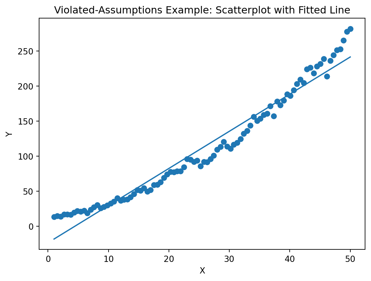
[1] Standard Errors assume that the covariance matrix of the errors is correctly specified.Scatterplot with fitted line
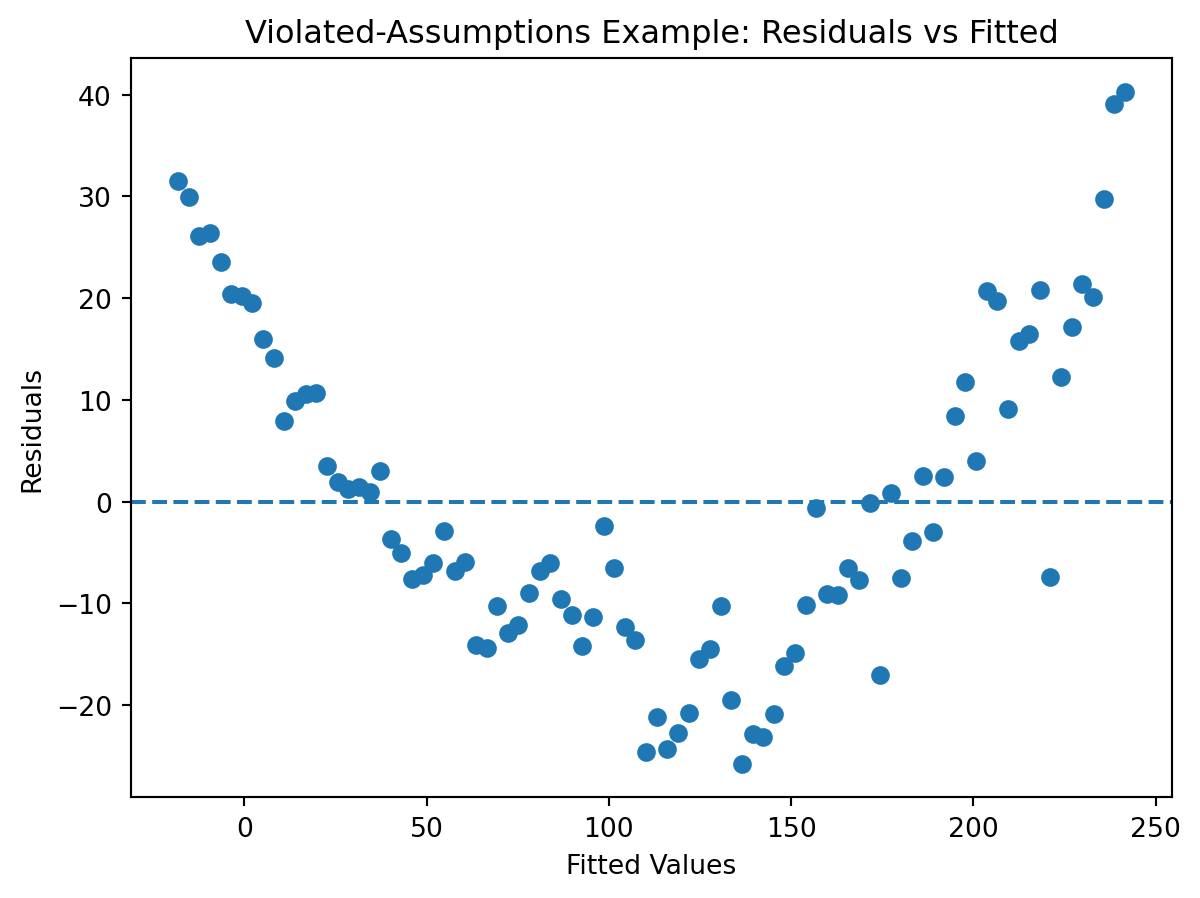
Residuals versus fitted
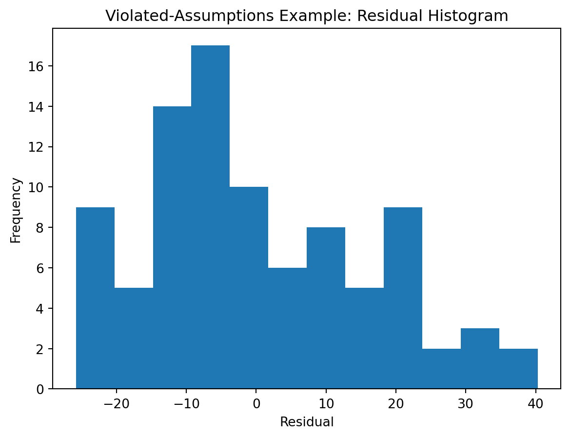
Histogram of residuals
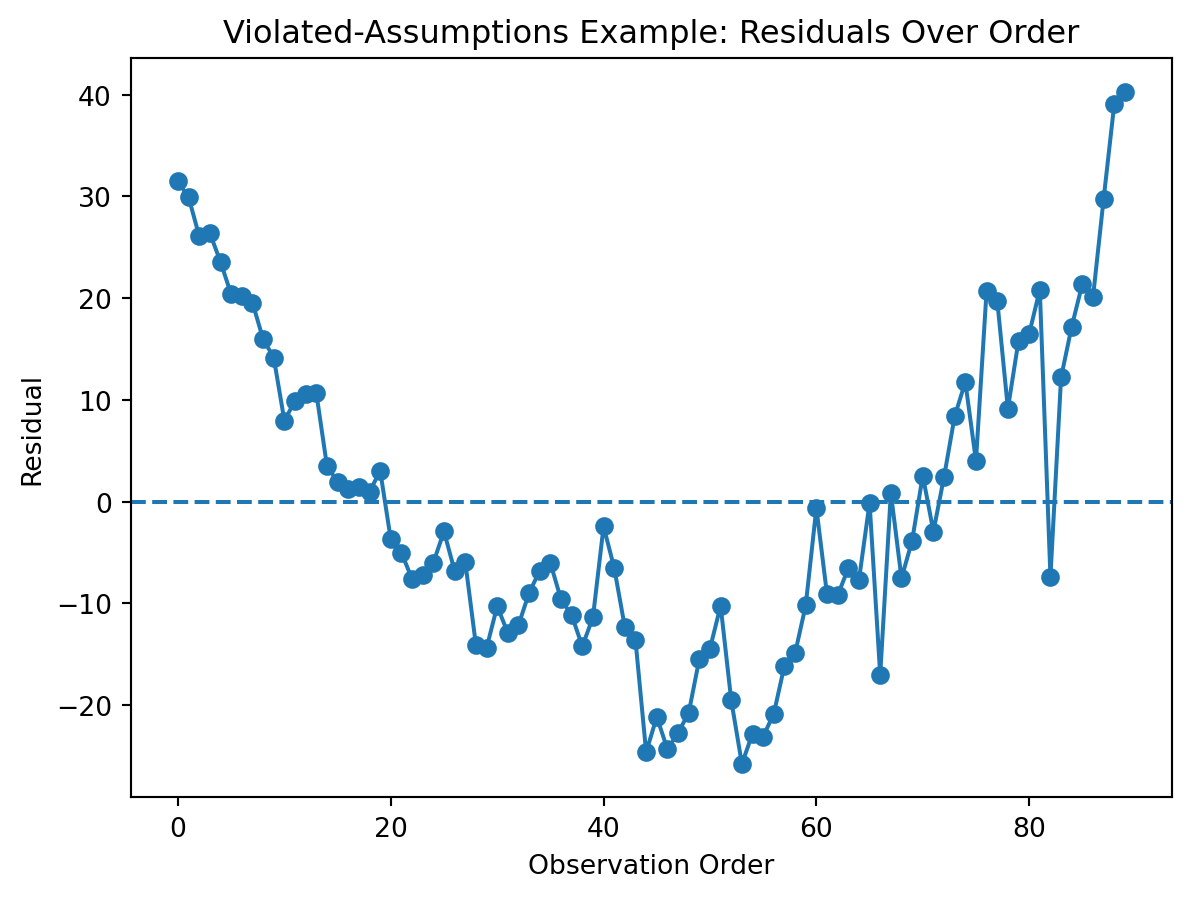
Residuals over observation order
How a student should read this violated example
A student should be able to say something like:
The scatterplot suggests that the relationship may be curved, so a straight line may not be appropriate. The residuals versus fitted plot shows a pattern rather than a random cloud, which suggests a violation of linearity. The spread of the residuals also appears to change, which raises concern about non-constant variance. The residual histogram is less well-behaved than in the earlier example, so normality is more questionable. The residuals over order show run-like behavior, suggesting correlation across observations. Overall, this model would need more caution and possibly a different modeling approach.
12. Step-by-Step in JMP: How to Check Assumptions
Fit the model first
- Open your dataset in JMP.
- Go to Analyze.
- Choose Fit Y by X for a simple regression, or Fit Model for broader modeling.
- Put the outcome in Y and the predictor in X.
- Run the model.
Look at the scatterplot and fitted line
Students should ask: - Does the line look like a reasonable summary? - Is there visible curvature? - Are there obvious outliers?
Look at residual plots
In JMP, use the red triangle options to request residual-related output. Focus on: - Residual by Predicted Plot - residual patterns over order if relevant - unusual points or changing spread
Look at the distribution of residuals
If available, examine: - a histogram of residuals, - or a normal plot / Q-Q style plot.
Ask: - Is the residual distribution roughly centered near zero? - Does it look approximately symmetric? - Are there extreme tails or outliers?
Think about the data structure
Before trusting independence, ask: - Are observations collected over time? - Are there repeated measures on the same unit? - Are observations clustered?
That question is often just as important as any diagnostic plot.
13. Common Mistakes When Checking Assumptions
Mistake 1: Thinking assumptions must be perfectly true
Real data almost never behave perfectly. The question is whether the model is reasonable enough.
Mistake 2: Confusing normality of \(Y\) with normality of residuals
The assumption is about the residuals, not necessarily the raw variables.
Mistake 3: Ignoring problem structure
If the data come from time series or repeated measures, independence deserves special attention.
Mistake 4: Looking only at tables and ignoring plots
Plots often reveal problems much more clearly than summary numbers.
Mistake 5: Treating every small imperfection as fatal
Minor deviations are common. We worry more about strong, systematic violations.
Mistake 6: Forgetting that diagnostics happen after the model is fit
Assumption checking is usually post hoc. Students should not expect to prove the assumptions first and then fit the model second.
14. Check Your Understanding
Questions
Why is assumption checking usually described as a post hoc process?
What is a residual, and how is it calculated?
What does the linearity assumption mean in plain language?
In a residual histogram, what should you generally hope to see?
Why are normal residuals mainly important for inference rather than for simply drawing a line?
What does a funnel-shaped residual plot suggest?
How can non-constant variance affect p-values and confidence intervals?
Which plot is most useful for checking constant variance?
Why is independence often connected to the structure of the problem?
Give two examples of settings where uncorrelated residuals may be less plausible.
If residuals show a strong curved pattern, which assumption is most likely being violated?
If the residual histogram is somewhat imperfect but the sample is fairly large, should you automatically reject the model?
Suggested answers
TipReveal suggested answers
1. Why is assumption checking usually described as a post hoc process?
Because we usually fit the model first and then examine the residuals and diagnostic plots afterward.
2. What is a residual, and how is it calculated?
A residual is the difference between the actual observed value and the predicted value from the model: actual minus predicted.
3. What does the linearity assumption mean in plain language?
It means a straight line is a reasonably good summary of the average relationship between \(X\) and \(Y\).
4. In a residual histogram, what should you generally hope to see?
A distribution roughly centered around zero, reasonably symmetric, and without extreme strange tails or isolated outliers.
5. Why are normal residuals mainly important for inference rather than for simply drawing a line?
Because normality affects how reliable the usual p-values, t-tests, and confidence intervals are, especially in smaller samples.
6. What does a funnel-shaped residual plot suggest?
It suggests non-constant variance, also called heteroscedasticity.
7. How can non-constant variance affect p-values and confidence intervals?
It can distort standard errors, which can then make p-values and confidence intervals misleading.
8. Which plot is most useful for checking constant variance?
The residuals versus fitted values plot.
9. Why is independence often connected to the structure of the problem?
Because dependence often comes from how the data were collected, such as time ordering, repeated measures, or clustering.
10. Give two examples of settings where uncorrelated residuals may be less plausible.
Time series data and repeated measures on the same person, store, or company.
11. If residuals show a strong curved pattern, which assumption is most likely being violated?
The linearity assumption.
12. If the residual histogram is somewhat imperfect but the sample is fairly large, should you automatically reject the model?
No. The key question is whether the deviation is serious enough to undermine useful inference or interpretation.
15. Key Takeaways
ImportantWhat to remember from this section
- Assumption checking is usually a post hoc part of regression analysis
- Residuals are the actual minus predicted values and are central to diagnostics
- Linearity is about whether a straight line is a good summary
- Normal residuals should be roughly centered near zero and mainly matter for p-values and confidence intervals
- Constant variance matters because changing spread can distort standard errors and other uncertainty measures
- Uncorrelated residuals often depend on the structure of the problem, especially in time series and repeated measures settings
- Residual plots are among the most useful diagnostic tools in regression
16. Looking Ahead
Once students understand assumptions and diagnostics, they are much better prepared to interpret regression output responsibly.
This also sets up the next major idea in analytics:
A model is not just something to fit. It is something to question.