flowchart LR
    A[Scatterplot of Data] --> B[Fit a Line]
    B --> C[Interpret the Slope]
    C --> D[Make Predictions Carefully]
Part 2: Modeling One Relationship — Simple Linear Regression
ImportantThe goal of this section
Simple linear regression helps us move beyond asking whether two variables are related and begin asking a deeper question:
How much does one variable tend to change when another variable changes?
This makes regression one of the most useful tools in analytics for decision-making.
2.1 Why Simple Linear Regression Matters
Correlation tells us whether two variables move together and how strongly they do so in a linear way. That is useful, but it is limited.
A manager rarely wants only this answer:
“Advertising and sales are positively related.”
A more useful question is:
“How much do sales tend to change when advertising changes?”
That is where simple linear regression becomes helpful.
Simple linear regression gives us a way to:
- describe a relationship with an equation,
- estimate the direction of the relationship,
- estimate the size of the relationship,
- make predictions,
- and begin translating data into action.
Example business questions
- How much does sales tend to increase when advertising spend rises?
- How much does demand tend to decrease when price rises?
- How much does customer spending tend to increase with income?
- How much does productivity tend to change as training hours increase?
Regression does not answer every question, and it does not automatically prove causality, but it gives a much richer answer than correlation alone.
2.2 From Scatterplot to Regression Line
A scatterplot shows the relationship between two variables. A regression line summarizes that relationship with a straight line.
The regression line is often called the line of best fit.
It is the straight line that best summarizes the overall linear pattern in the data.
Below is a simulated example.
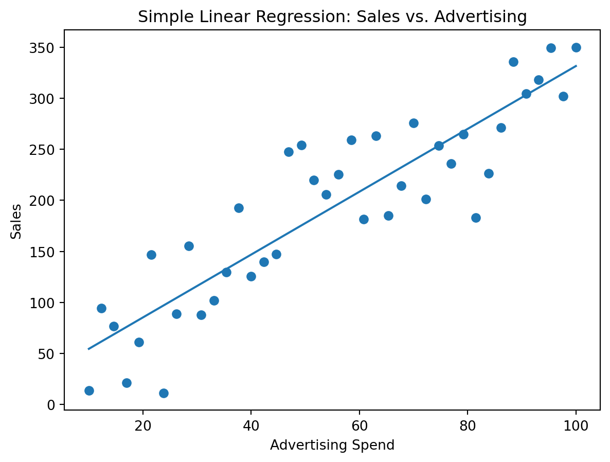
The points represent observed data. The line is the model’s summary of the average linear relationship.
A regression line will almost never pass through every point. That is normal. Real data contain noise, variation, and factors not included in the model.
2.3 The Regression Equation
A simple linear regression model is usually written as:
\[ Y = \beta_0 + \beta_1 X + \varepsilon \]
This looks mathematical, but the ideas behind it are very manageable.
What each part means
- \(Y\) = the outcome or dependent variable
- \(X\) = the predictor or explanatory variable
- \(\beta_0\) = the intercept
- \(\beta_1\) = the slope
- \(\varepsilon\) = the error term, or the part not explained by the model
In estimated form, we often write:
\[ \hat{Y} = b_0 + b_1 X \]
where:
- \(\hat{Y}\) is the predicted value of \(Y\),
- \(b_0\) is the estimated intercept,
- \(b_1\) is the estimated slope.
A plain-language interpretation
If the fitted equation is:
\[ \widehat{Sales} = 20 + 3.2(Advertising) \]
then:
- the intercept is 20,
- the slope is 3.2.
This means the model predicts that, on average, sales increase by about 3.2 units for each 1-unit increase in advertising.
That slope is usually the most important quantity in simple linear regression.
2.4 What the Slope Means
The slope tells us the expected change in the outcome variable for a one-unit increase in the predictor variable.
That sounds technical, so let’s slow it down.
If the slope is 3.2, then:
- when \(X\) increases by 1,
- predicted \(Y\) increases by 3.2, on average.
Business translation
If: - \(X\) = advertising spend in thousands of dollars - \(Y\) = sales in thousands of dollars
and the slope is 3.2, then:
For each additional $1,000 of advertising, predicted sales increase by about $3,200 on average.
This does not necessarily prove advertising caused the increase. But it gives a concrete, interpretable estimate of the relationship in the data.
ImportantMost important idea
In simple linear regression, the slope is usually the first number you should try to interpret in business language.
2.5 What the Intercept Means
The intercept is the predicted value of \(Y\) when \(X = 0\).
In the example:
\[ \widehat{Sales} = 20 + 3.2(Advertising) \]
the intercept of 20 means:
predicted sales are 20 when advertising is 0.
Sometimes that is meaningful. Sometimes it is not.
Why the intercept can be tricky
If \(X = 0\) is realistic and falls within the data range, the intercept may be interpretable.
But if \(X = 0\) is unrealistic or far outside the observed data, the intercept is often just a mathematical anchor for the line and should not be overinterpreted.
Note
Intercepts are often less interesting than slopes in business settings.
2.6 How the Line Is Chosen: Residuals
A regression line is not drawn by eye. It is chosen to fit the data mathematically.
The model does this by trying to make the prediction errors as small as possible.
A residual is:
\[ \text{Residual} = \text{Actual Value} - \text{Predicted Value} \]
So each point has: - an actual \(Y\) value, - a predicted \(Y\) value from the line, - and a difference between the two.
The model picks the line that minimizes the sum of the squared residuals. That is why this is often called least squares regression.
Visualizing residuals
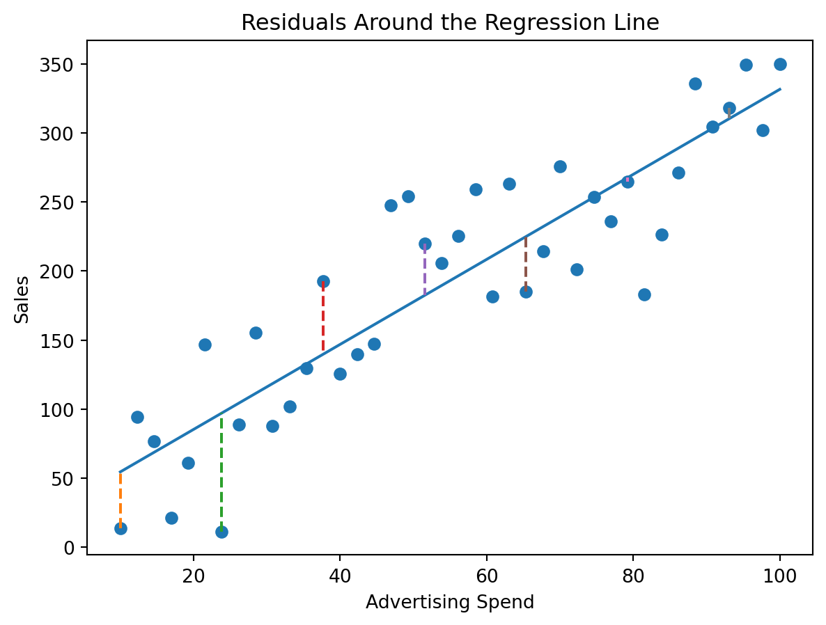
The dashed vertical distances show the residuals for a sample of points. Some points fall above the line and some below it.
That is expected. A model is not meant to explain everything perfectly.
2.7 Making Predictions with the Regression Line
Once we have a fitted equation, we can use it to make predictions.
Suppose the fitted model is:
\[ \widehat{Sales} = 20 + 3.2(Advertising) \]
If advertising = 50, then:
\[ \widehat{Sales} = 20 + 3.2(50) = 180 \]
So the model predicts sales of 180.
That is a useful business capability. But prediction still requires care.
A good rule
Predictions are usually more trustworthy when they are made within the range of the observed data.
If your data only include advertising values from 10 to 100, then using the model to predict at 500 is risky. That is called extrapolation, and it can be very misleading.
Warning
A regression model is most trustworthy in the region where you actually have data.
2.8 R-Squared: How Much Variation Is Explained?
One of the most common regression outputs is \(R^2\).
This measures the proportion of variation in the outcome variable that is explained by the model.
Interpretation
- \(R^2 = 0\) means the model explains none of the variation
- \(R^2 = 1\) means the model explains all of the variation
Example
If \(R^2 = 0.64\), that means:
About 64% of the variation in \(Y\) is explained by \(X\) in this model.
That can be helpful, but it must be interpreted carefully.
How \(R^2\) relates to \(r\) in simple linear regression
In a simple linear regression with one predictor, there is a special relationship:
\[ R^2 = r^2 \]
where: - \(r\) is the Pearson correlation between \(X\) and \(Y\), - and \(R^2\) is the regression model’s explained proportion of variation.
So if the correlation is:
\[ r = 0.80 \]
then:
\[ R^2 = 0.80^2 = 0.64 \]
That means a correlation of 0.80 corresponds to 64% of the variation being explained in a simple linear regression.
Note
This special relationship holds for simple linear regression with one predictor. Once we move to multiple regression, \(R^2\) is no longer just the square of one correlation.
What R-squared does NOT tell you
\(R^2\) does not tell you: - whether the relationship is causal, - whether the model is appropriate, - whether the predictions are good enough for a decision, - or whether important variables are missing.
A model can have a decent \(R^2\) and still be poor for decision-making.
2.9 Simulated Example: Stronger vs Weaker Fit
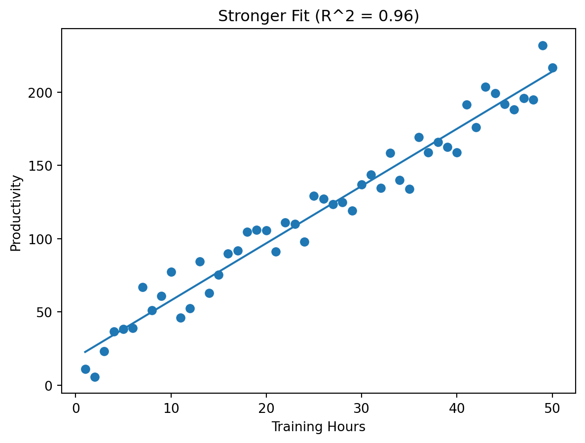
Below are two simulated datasets with different levels of noise.
Example A: Stronger fit
Example B: Weaker fit
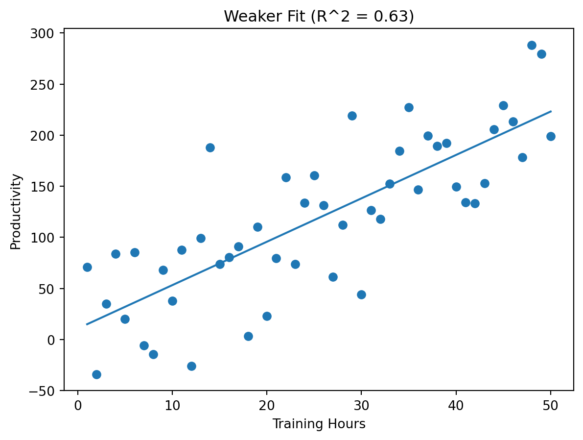
In both cases the relationship is positive, but the first model is clearly tighter and explains more variation.
This is a useful reminder:
The slope tells you the direction and size of the relationship.
\(R^2\) tells you how tightly the data cluster around that relationship.
2.10 P-Values and Hypothesis Testing
Another common regression output is the p-value.
A p-value does not stand alone. It is the result of a hypothesis test.
In simple linear regression, the most important hypothesis test usually concerns the slope.
The hypothesis test for the slope
The model is often testing:
\[ H_0: \beta_1 = 0 \]
versus
\[ H_A: \beta_1 \neq 0 \]
In plain language, that means:
- Null hypothesis (\(H_0\)): there is no linear relationship between \(X\) and \(Y\) in the population
- Alternative hypothesis (\(H_A\)): there is a linear relationship between \(X\) and \(Y\) in the population
What the p-value means
The p-value tells us how compatible the observed sample evidence is with the null hypothesis.
A small p-value means the observed slope would be unlikely if the true slope were actually zero.
Compare the p-value to alpha
The p-value should be compared to alpha, the significance level chosen in advance.
Common choices are:
- \(\alpha = 0.05\)
- \(\alpha = 0.01\)
The decision rule is:
- if p-value \(\le \alpha\), reject the null hypothesis
- if p-value \(> \alpha\), fail to reject the null hypothesis
Practical interpretation
If the p-value for the slope is 0.02 and alpha is 0.05, then:
- 0.02 is less than 0.05,
- so we reject the null hypothesis,
- and conclude that the slope is statistically significant at the 5% level.
That means the data provide evidence of a linear relationship between \(X\) and \(Y\).
ImportantWhich p-value matters most?
To decide whether the relationship is statistically significant in simple linear regression, students should focus on the p-value for the slope, not the p-value for the intercept.
Why the intercept p-value is usually not the key question
The intercept test asks whether the predicted value of \(Y\) when \(X = 0\) is different from zero.
That is often not the main business question.
In most simple linear regression problems, the central question is:
Does \(Y\) change as \(X\) changes?
That question is answered by the slope, not the intercept.
What significance does NOT mean
A statistically significant slope does not mean: - the effect is large, - the effect is important, - the relationship is causal, - or the model is useful in practice.
Warning
Do not confuse “statistically significant” with “managerially important.”
A very small effect can be statistically significant in a large sample. A meaningful effect can fail to be statistically significant in a small sample.
2.11 Confidence Intervals for the Slope
A confidence interval gives a plausible range for the true slope.
For example, if the slope estimate is 3.2 and the 95% confidence interval is:
- 2.1 to 4.3
then a careful interpretation is:
Based on the sample, the true average increase in \(Y\) for a one-unit increase in \(X\) is plausibly between 2.1 and 4.3.
This is often more informative than looking only at a p-value because it tells you both: - the likely direction, - and the likely size of the effect.
2.12 What JMP Output Typically Means
When students run simple linear regression in JMP, they will often see output that includes:
- a scatterplot and fitted line,
- parameter estimates,
- an \(R^2\) value,
- p-values for coefficients,
- and residual information.
The main pieces students should learn to read
1. The fitted equation
This tells you the intercept and slope.
2. The slope estimate
This tells you how much \(Y\) is predicted to change when \(X\) changes by one unit.
3. The p-value for the slope
This is the main p-value used to assess whether the relationship is statistically significant.
4. The intercept p-value
This may appear in the table, but it is usually not the main basis for deciding whether the relationship itself is significant.
5. \(R^2\)
This tells you how much of the variation in \(Y\) is explained by \(X\).
6. The graph
This helps you check: - whether the relationship looks linear, - whether outliers are present, - and whether the fitted line seems to summarize the data reasonably well.
2.13 Simulated Output Table: How to Read It
Below is a simplified example of the type of regression output students may see.
| Term | Estimate | p-value | Interpretation |
|---|---|---|---|
| Intercept | 20.0 | 0.180 | Predicted \(Y\) when \(X = 0\) |
| X Variable | 3.2 | 0.001 | Predicted change in \(Y\) for a 1-unit increase in \(X\) |
| Model Summary | Value |
|---|---|
| \(R^2\) | 0.64 |
| Alpha | 0.05 |
How to interpret this output
A student should be able to say something like:
The estimated regression equation suggests that \(Y\) increases by about 3.2 units for each 1-unit increase in \(X\). The p-value for the slope is 0.001, which is below alpha = 0.05, so the slope is statistically significant. The intercept p-value is not the main test of whether the relationship exists. The model explains about 64% of the variation in \(Y\), which suggests a moderately strong fit. However, this does not by itself prove a causal effect.
That kind of explanation is much stronger than simply reading the table aloud.
2.14 A Full Simulated Example with Actual Python Output
Below is a complete worked example. The goal is not to teach coding, but to show what real output looks like and how to interpret it.
Scenario
Suppose a company wants to understand the relationship between advertising spend and monthly sales.
We will simulate data where: - advertising is the predictor, - sales is the outcome, - and there is a positive relationship plus random noise.
import numpy as np
import pandas as pd
import statsmodels.api as sm

np.random.seed(2026)

advertising = np.random.uniform(10, 100, 60)
sales = 25 + 2.8 * advertising + np.random.normal(0, 30, 60)

df = pd.DataFrame({
    "advertising": advertising,
    "sales": sales
})

X = sm.add_constant(df["advertising"])
model = sm.OLS(df["sales"], X).fit()

print(model.summary())
OLS Regression Results
==============================================================================
Dep. Variable: sales R-squared: 0.868
Model: OLS Adj. R-squared: 0.866
Method: Least Squares F-statistic: 381.5
Date: Tue, 07 Apr 2026 Prob (F-statistic): 3.49e-27
Time: 16:03:26 Log-Likelihood: -286.01
No. Observations: 60 AIC: 576.0
Df Residuals: 58 BIC: 580.2
Df Model: 1
Covariance Type: nonrobust
===============================================================================
coef std err t P>|t| [0.025 0.975]
-------------------------------------------------------------------------------
const 31.0195 8.198 3.784 0.000 14.610 47.429
advertising 2.7213 0.139 19.531 0.000 2.442 3.000
==============================================================================
Omnibus: 9.418 Durbin-Watson: 2.182
Prob(Omnibus): 0.009 Jarque-Bera (JB): 11.488
Skew: -0.607 Prob(JB): 0.00320
Kurtosis: 4.767 Cond. No. 129.
==============================================================================
Notes:
[1] Standard Errors assume that the covariance matrix of the errors is correctly specified.Visualizing the simulated data
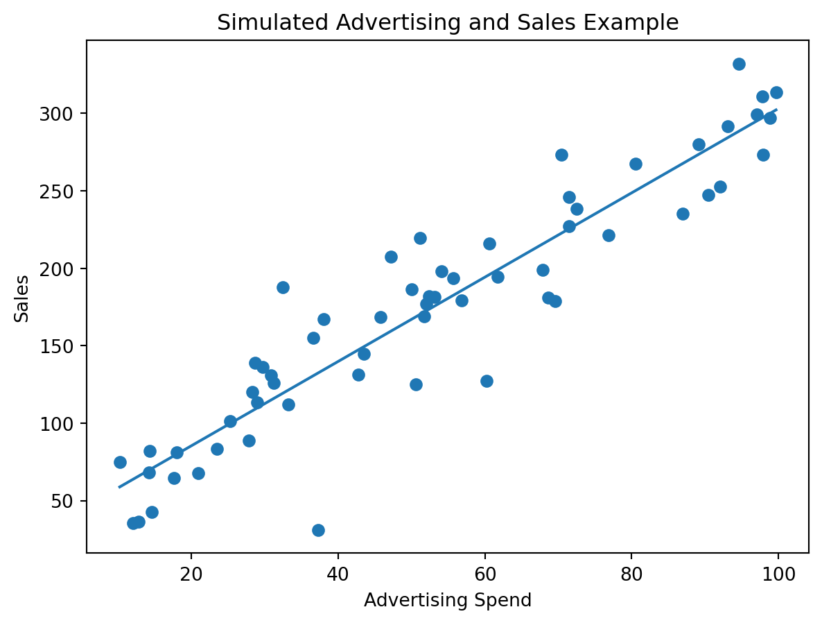
Questions about the output
When students look at the printed output, they should try to answer questions like these:
- Is the estimated slope positive or negative?
- What does the slope mean in business terms?
- Is the slope statistically significant at alpha = 0.05?
- Should the p-value for the intercept be used to determine whether the relationship exists?
- What does \(R^2\) say about model fit?
- Does this model prove that advertising causes sales to increase?
Suggested answers
TipReveal suggested answers
1. Is the estimated slope positive or negative?
It should be positive, because the data were simulated with a positive relationship between advertising and sales.
2. What does the slope mean in business terms?
It tells us how much sales are predicted to change, on average, for a 1-unit increase in advertising spend.
3. Is the slope statistically significant at alpha = 0.05?
Students should compare the p-value for the slope to 0.05. If the p-value is less than or equal to 0.05, then the slope is statistically significant.
4. Should the p-value for the intercept be used to determine whether the relationship exists?
No. The relationship is assessed primarily by the p-value for the slope.
5. What does \(R^2\) say about model fit?
It tells us the proportion of variation in sales explained by advertising in this simple linear regression.
6. Does this model prove that advertising causes sales to increase?
No. It shows an estimated linear relationship in the data, but that alone does not prove causality.
2.15 Step-by-Step in JMP: Running Simple Linear Regression
There are multiple ways to explore a simple relationship in JMP, but one of the most useful is Fit Y by X.
Option 1: Analyze > Fit Y by X
- Open your dataset in JMP.
- Go to Analyze.
- Choose Fit Y by X.
- Put the outcome variable in Y, Response.
- Put the predictor variable in X, Factor.
- Click OK.
If both variables are continuous, JMP will create a bivariate fit.
From there, you can: - view the scatterplot, - inspect the overall pattern, - and use the red triangle menu to add the fitted line and additional output.
Add the linear fit
After the bivariate plot appears:
- Click the red triangle next to Bivariate Fit of Y By X.
- Choose Fit Line.
This will typically provide: - the regression line, - parameter estimates, - an \(R^2\) value, - an analysis of variance summary, - and tests for the slope.
What to look for in JMP
Students should focus on these questions:
- Is the fitted line upward or downward?
- What does the slope mean in context?
- What is the p-value for the slope, and how does it compare to alpha?
- Is the relationship statistically significant?
- How much variation is explained?
- Are there outliers or obvious nonlinear patterns?
- Does the line seem like a sensible summary of the data?
Option 2: Graph Builder for visual exploration
You can also begin with:
- Graph
- Graph Builder
- Place X on the horizontal axis
- Place Y on the vertical axis
This is useful for a quick visual inspection before fitting the line formally.
2.16 Common Mistakes in Simple Linear Regression
Students often make the same interpretation mistakes repeatedly. Here are some of the most important ones.
Mistake 1: Treating slope as proof of causality
A positive slope does not prove \(X\) causes \(Y\).
Mistake 2: Ignoring units
A slope only makes sense if you interpret it using the units of \(X\) and \(Y\).
Mistake 3: Overinterpreting the intercept
The intercept may not be meaningful if \(X = 0\) is unrealistic.
Mistake 4: Trusting \(R^2\) too much
A higher \(R^2\) does not guarantee a good or useful model.
Mistake 5: Predicting far outside the data range
Extrapolation can produce misleading conclusions.
Mistake 6: Ignoring the graph
A regression table is useful, but the graph often reveals problems the numbers hide.
Mistake 7: Looking at the wrong p-value
Students sometimes focus on the intercept p-value when the real question is whether the slope is statistically different from zero.
2.17 Mini Case: Advertising and Sales
NoteScenario
A company fits a simple linear regression model relating monthly advertising spend to monthly sales. The estimated equation is:
\[ \widehat{Sales} = 20 + 3.2(Advertising) \]
The slope p-value is 0.001, alpha is 0.05, and \(R^2 = 0.64\).
Questions to ask
- What does the slope mean in business terms?
- Is the slope statistically significant at the chosen alpha level?
- Is 64% explained variation strong enough to be useful?
- Does this result prove that increasing advertising will cause higher sales?
- Could seasonality or promotions be influencing both variables?
A strong student interpretation
A strong answer might sound like this:
The model suggests that sales increase by about 3.2 units for each additional unit of advertising, on average. Because the slope p-value is 0.001 and alpha is 0.05, the slope is statistically significant. The model explains a meaningful share of sales variation. However, the result alone does not prove a causal effect because other factors may be influencing both advertising and sales.
That is the kind of language students should aim for.
2.18 Check Your Understanding
Questions
What is the main difference between correlation and simple linear regression?
In the equation \(\hat{Y} = b_0 + b_1 X\), what does the slope represent?
What does the intercept represent, and why can it sometimes be hard to interpret?
What is a residual?
What does \(R^2\) measure?
In simple linear regression, how does \(R^2\) relate to \(r\)?
What hypothesis is usually being tested when we examine the p-value for the slope?
Why should the p-value be compared to alpha?
Which p-value determines whether the relationship is statistically significant: the slope p-value or the intercept p-value?
Why should analysts be cautious about claiming causality from a simple linear regression?
Suggested answers
TipReveal suggested answers
1. What is the main difference between correlation and simple linear regression?
Correlation summarizes the strength and direction of a linear relationship. Simple linear regression goes further by fitting an equation that quantifies how \(Y\) changes as \(X\) changes.
2. In the equation \(\hat{Y} = b_0 + b_1 X\), what does the slope represent?
It represents the predicted change in \(Y\) for a one-unit increase in \(X\).
3. What does the intercept represent, and why can it sometimes be hard to interpret?
It is the predicted value of \(Y\) when \(X = 0\). It can be hard to interpret if \(X = 0\) is unrealistic or outside the observed data range.
4. What is a residual?
A residual is the difference between the actual observed value of \(Y\) and the value predicted by the regression line.
5. What does \(R^2\) measure?
It measures the proportion of variation in \(Y\) explained by the model.
6. In simple linear regression, how does \(R^2\) relate to \(r\)?
In simple linear regression, \(R^2 = r^2\), where \(r\) is the Pearson correlation between \(X\) and \(Y\).
7. What hypothesis is usually being tested when we examine the p-value for the slope?
The null hypothesis is that the true slope equals zero, meaning no linear relationship in the population.
8. Why should the p-value be compared to alpha?
Because alpha is the decision threshold chosen in advance. The p-value only becomes meaningful for decision-making when compared to that threshold.
9. Which p-value determines whether the relationship is statistically significant: the slope p-value or the intercept p-value?
The slope p-value.
10. Why should analysts be cautious about claiming causality from a simple linear regression?
Because omitted variables, reverse causality, and other explanations may account for the observed relationship.
2.19 Key Takeaways
ImportantWhat to remember from Part 2
- Simple linear regression models the relationship between one predictor and one outcome
- The slope is usually the most important quantity to interpret
- The intercept is the predicted value when \(X = 0\), but it is not always meaningful
- Residuals measure how far points are from the fitted line
- In simple linear regression, \(R^2 = r^2\)
- The p-value comes from a hypothesis test and should be compared to alpha
- The slope p-value, not the intercept p-value, is the key test of whether the relationship is statistically significant
- Statistical significance does not guarantee practical importance
- Regression can support decisions, but it does not automatically prove causality
2.20 Looking Ahead
In the next section, we move to multiple linear regression.
That will allow us to study what happens when more than one variable may help explain the outcome, and why “holding other things constant” is one of the most important ideas in analytics.