Part 3: Multiple Linear Regression — Controlling for More Than One Factor

ImportantThe goal of this section

Simple linear regression asks:

How does one predictor relate to one outcome?

Multiple linear regression asks a more realistic business question:

How does each predictor relate to the outcome after accounting for the other predictors in the model?

That idea — holding other variables constant — is what makes multiple regression so powerful and so important for business decision-making.

---

3.1 Why Multiple Linear Regression Matters

Real business outcomes are almost never driven by just one variable.

For example, sales may depend on:

• advertising,
• price,
• promotions,
• store size,
• seasonality,
• and local competition.

If we look at advertising alone, we may confuse its effect with the effects of the other variables.

Multiple linear regression helps us separate these influences more carefully.

Example business questions

• What is the relationship between advertising and sales after controlling for price and promotions?
• Does training still matter after controlling for prior performance and experience?
• Does price affect demand after controlling for product category and season?

Note

Multiple regression is often less about finding “the one best predictor” and more about understanding which variables still matter after accounting for others.

---

3.2 How Multiple Regression Differs from Simple Regression

In simple linear regression, we model one predictor and one outcome:

\[ Y = \beta_0 + \beta_1 X + \varepsilon \]

In multiple linear regression, we model several predictors at once:

\[ Y = \beta_0 + \beta_1 X_1 + \beta_2 X_2 + \cdots + \beta_k X_k + \varepsilon \]

Key difference in interpretation

In simple regression, the slope tells us how \(Y\) changes with \(X\) when \(X\) is the only predictor in the model.

In multiple regression, each slope tells us how \(Y\) changes with that predictor holding the other predictors constant.

That is a big change.

Why this matters

A variable may appear important in a simple regression because it is related to: - the outcome, - another important predictor, - or both.

Once other predictors are added, that variable’s coefficient and p-value may change substantially.

This is not a bug. It is one of the most important lessons in regression.

---

3.3 The Basic Multiple Regression Equation

A multiple linear regression model is usually written as:

\[ Y = \beta_0 + \beta_1 X_1 + \beta_2 X_2 + \cdots + \beta_k X_k + \varepsilon \]

In estimated form:

\[ \hat{Y} = b_0 + b_1 X_1 + b_2 X_2 + \cdots + b_k X_k \]

where:

• \(Y\) = the outcome variable
• \(X_1, X_2, \ldots, X_k\) = predictors
• \(\beta_0\) = the population intercept
• \(\beta_1, \beta_2, \ldots, \beta_k\) = population slopes
• \(\varepsilon\) = the error term
• \(\hat{Y}\) = predicted value of \(Y\)

Example

Suppose we model sales as a function of advertising, price, and promotion:

\[ \widehat{Sales} = 50 + 2.1(Advertising) - 3.4(Price) + 12.0(Promotion) \]

Then:

• the intercept is 50,
• the advertising coefficient is 2.1,
• the price coefficient is -3.4,
• the promotion coefficient is 12.0.

Interpretation

• For a one-unit increase in advertising, predicted sales increase by 2.1 holding price and promotion constant
• For a one-unit increase in price, predicted sales decrease by 3.4 holding advertising and promotion constant
• If promotion changes by one unit, predicted sales increase by 12.0 holding the other predictors constant

ImportantCore interpretation rule

In multiple regression, every slope is interpreted conditional on the other variables in the model.

---

3.4 Why Coefficients Change When Variables Are Added

One of the most important differences between simple and multiple regression is that coefficients can change when new predictors are added.

Why does this happen?

Because predictors often overlap in the information they contain.

For example: - advertising may be higher during promotions, - price may vary by product category, - training hours may be higher for already stronger employees.

If two predictors are related to each other, the model must decide how much of the outcome each one explains.

That can cause: - coefficient estimates to change, - p-values to change, - and even the sign of a coefficient to change in some cases.

Intuition

In simple regression, a predictor may capture: - its own effect, - plus some of the effect of omitted variables correlated with it.

Once those omitted variables are added, the coefficient can move closer to its more conditional interpretation.

This is one reason simple regression can be misleading if important predictors are left out.

---

3.5 A Visual Intuition for Multiple Regression

With one predictor, we can draw a line on a scatterplot.

With two predictors, the fitted relationship becomes a plane in 3D.

With more than two predictors, the geometry becomes harder to visualize directly, but the idea is the same: the model is estimating the average outcome as a function of multiple inputs at once.

flowchart LR
    A[Simple Regression: One X] --> B[One Slope]
    B --> C[Multiple Regression: Many Xs]
    C --> D[Each Slope Is Conditional on the Others]

This is why multiple regression often gives more realistic business insight than simple regression.

---

3.6 Simulated Example: Simple vs Multiple Regression

Below is a simulated example where sales depend on advertising and price.

A simple regression view

Simple regression of sales on advertising only.

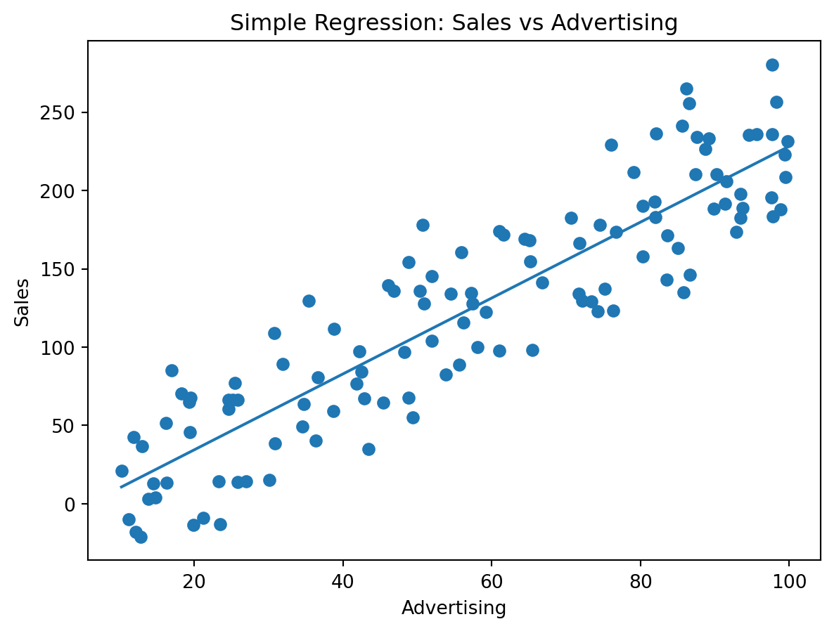
This simple relationship may look meaningful, but it ignores price and promotion.

Output comparison

print("Simple regression coefficients:")
print(model_simple.params)
print()
print("Multiple regression coefficients:")
print(model_multi.params)

Simple regression coefficients:
const         -13.989163
advertising     2.422173
dtype: float64

Multiple regression coefficients:
const          50.820740
advertising     2.450220
price          -4.569148
promotion       5.450684
dtype: float64

What students should notice

The advertising coefficient in the simple model will usually not exactly match the advertising coefficient in the multiple model.

That is because:

• the simple model ignores price and promotion,
• the multiple model adjusts for them,
• so the advertising slope in the multiple model is more conditional.

---

3.7 Interpreting Multiple Regression Output

When students look at multiple regression output, the key pieces are similar to simple regression, but the interpretation is more careful.

Main output pieces

• coefficient estimates,
• standard errors,
• t-statistics,
• p-values,
• confidence intervals,
• \(R^2\) and adjusted \(R^2\).

Example coefficient table

Predictor	Estimate	p-value	Interpretation
Intercept	50.0	0.120	Predicted sales when all predictors are 0
Advertising	2.1	0.001	Change in sales for a 1-unit increase in advertising, holding other predictors constant
Price	-3.4	0.004	Change in sales for a 1-unit increase in price, holding other predictors constant
Promotion	12.0	0.030	Difference in sales associated with promotion, holding the other predictors constant

A strong student interpretation

Holding price and promotion constant, a one-unit increase in advertising is associated with an average increase of 2.1 units in sales. Holding advertising and promotion constant, a one-unit increase in price is associated with an average decrease of 3.4 units in sales. Promotion is also associated with higher sales after accounting for the other predictors.

That kind of interpretation is much stronger than saying only “advertising is significant.”

---

3.8 What the P-Values Mean in Multiple Regression

Each p-value in a multiple regression is tied to a hypothesis test.

For predictor \(X_j\), the usual test is:

\[ H_0: \beta_j = 0 \]

versus

\[ H_A: \beta_j \neq 0 \]

Interpretation

The p-value for a predictor asks:

Is there evidence that this predictor is related to the outcome after accounting for the other predictors already in the model?

This is the most important difference from simple regression.

A variable can be significant in a simple regression but not significant in a multiple regression if its apparent effect overlaps with other predictors.

Compare to alpha

As before, the p-value should be compared to alpha, such as:

• \(\alpha = 0.05\)
• \(\alpha = 0.01\)

Decision rule: - if p-value \(\le \alpha\), reject \(H_0\) - if p-value \(> \alpha\), fail to reject \(H_0\)

ImportantImportant interpretation rule

In multiple regression, the p-value for a variable reflects its contribution given the other variables in the model.

---

3.9 Why P-Values Change When Variables Are Added or Deleted

This is one of the biggest sources of confusion for students.

A variable’s p-value can change when: - another predictor is added, - a predictor is removed, - or the model structure changes.

Why?

Because the coefficient estimate and its standard error both depend on: - which other variables are included, - how correlated those variables are, - and how much overlapping information they contain.

Common scenarios

Scenario 1: A variable loses significance after another is added

This often happens when the new variable explains much of the same variation.

Scenario 2: A variable becomes significant after another is removed

This can happen because the overlap and instability in the model changes.

Scenario 3: A coefficient changes sign

This can happen when omitted-variable issues or strong correlations among predictors are present.

Key lesson

A p-value is not a permanent property of a variable.

It is a property of a variable within a particular model.

Warning

Students should never say, “This variable is significant” without understanding that significance depends on what else is in the model.

---

3.10 Simulated Example: P-Values Change Across Models

Below is a comparison of a few different models using the same data.

X_m1 = sm.add_constant(df[["advertising"]])
m1 = sm.OLS(df["sales"], X_m1).fit()

X_m2 = sm.add_constant(df[["advertising", "price"]])
m2 = sm.OLS(df["sales"], X_m2).fit()

X_m3 = sm.add_constant(df[["advertising", "price", "promotion"]])
m3 = sm.OLS(df["sales"], X_m3).fit()

comparison = pd.DataFrame({
    "Model 1 coef": m1.params,
    "Model 1 p": m1.pvalues,
    "Model 2 coef": m2.params.reindex(m1.params.index.union(m2.params.index)),
    "Model 2 p": m2.pvalues.reindex(m1.params.index.union(m2.params.index)),
    "Model 3 coef": m3.params.reindex(m1.params.index.union(m2.params.index).union(m3.params.index)),
    "Model 3 p": m3.pvalues.reindex(m1.params.index.union(m2.params.index).union(m3.params.index))
})

print(comparison)

             Model 1 coef     Model 1 p  Model 2 coef     Model 2 p  \
advertising      2.422173  5.343111e-45      2.443432  5.117642e-70   
const          -13.989163  4.074470e-02     54.151470  1.464196e-15   
price                 NaN           NaN     -4.607752  4.103894e-30   
promotion             NaN           NaN           NaN           NaN   

             Model 3 coef     Model 3 p  
advertising      2.450220  5.988587e-70  
const           50.820740  3.749047e-13  
price           -4.569148  7.853667e-30  
promotion        5.450684  1.160587e-01  

What to look for

Students should ask:

• Does the advertising coefficient change across models?
• Does its p-value change?
• What happens to the model when price is added?
• What happens when promotion is added?

This is a great way to reinforce that coefficients and p-values are model-dependent.

---

3.11 Model Fit: \(R^2\) and Adjusted \(R^2\)

In multiple regression, \(R^2\) still measures the proportion of variation in \(Y\) explained by the model.

But now there is an important complication:

• adding more predictors can only increase \(R^2\) or leave it unchanged,
• even if the new predictors are not truly useful.

That is why adjusted \(R^2\) is often useful.

Adjusted \(R^2\)

Adjusted \(R^2\) penalizes the addition of predictors that do not help enough.

So:

• \(R^2\) rewards complexity,
• adjusted \(R^2\) rewards useful complexity.

Practical interpretation

A student might say:

The model with more variables has a higher \(R^2\), but we should also look at adjusted \(R^2\) to see whether the extra predictors improved the model enough to justify their inclusion.

---

3.12 What VIF Means

One major issue in multiple regression is that predictors can be strongly related to each other.

This is called multicollinearity.

A common diagnostic for this is the Variance Inflation Factor (VIF).

Basic idea

A VIF measures how much the variance of a coefficient is inflated because that predictor overlaps with the other predictors in the model.

Interpretation

• VIF = 1 → no inflation from correlation with other predictors
• VIF around 2 to 5 → some multicollinearity, often manageable
• VIF above 5 → potentially concerning
• VIF above 10 → often treated as a strong warning sign

These are rules of thumb, not absolute laws.

Why high VIF matters

High VIF can cause:

• unstable coefficients,
• larger standard errors,
• less reliable p-values,
• coefficients that change a lot across similar models,
• and difficulty interpreting individual predictors.

ImportantKey idea

High multicollinearity does not always hurt prediction badly, but it can make interpretation of individual coefficients much harder.

---

3.13 Simulated Example: Computing VIFs

Below is a simulated example where two predictors are intentionally related.

from statsmodels.stats.outliers_influence import variance_inflation_factor

np.random.seed(2028)

n_vif = 120
x1 = np.random.normal(size=n_vif)
x2 = 0.90 * x1 + np.random.normal(scale=0.35, size=n_vif)
x3 = np.random.normal(size=n_vif)
y_vif = 10 + 3*x1 + 2*x3 + np.random.normal(size=n_vif)

df_vif = pd.DataFrame({"x1": x1, "x2": x2, "x3": x3, "y": y_vif})

X_vif = sm.add_constant(df_vif[["x1", "x2", "x3"]])

vif_table = pd.DataFrame({
    "Variable": X_vif.columns,
    "VIF": [variance_inflation_factor(X_vif.values, i) for i in range(X_vif.shape[1])]
})

print(vif_table)

  Variable        VIF
0    const   1.089017
1       x1  10.387366
2       x2  10.364266
3       x3   1.010889

What students should notice

• \(x1\) and \(x2\) are strongly related
• their VIF values should be much higher than the VIF for \(x3\)
• that is a sign that interpreting their separate coefficients may be difficult

---

3.14 How to Deal with High VIF

If VIF is high, that does not automatically mean the model is unusable. It means students should think carefully.

Possible responses include:

1. Check whether the variables are conceptually redundant

Are two predictors measuring almost the same thing?

2. Remove one of the overlapping variables

This may improve interpretability, but only if the removed variable is not essential.

3. Combine variables

Sometimes related variables can be combined into: - an index, - an average, - or a composite measure.

4. Keep both if prediction is the main goal

If the goal is prediction rather than interpretation, multicollinearity can be less damaging.

5. Use judgment, not a mechanical rule

A high VIF is a warning sign, not an automatic delete command.

Note

Students should learn that variable selection is not just a math exercise. It is also a business judgment exercise.

---

3.15 A Practical Process for Getting to a Final Model

Students often want a clean step-by-step process. Here is a practical one.

Step 1: Start with the business question

What are we trying to explain or predict?

Step 2: Choose a reasonable initial set of predictors

Use domain knowledge and logic, not just convenience.

Step 3: Fit the model

Estimate coefficients, p-values, and fit measures.

Step 4: Check assumptions and diagnostics

Look at residual plots, outliers, and general model behavior.

Step 5: Check multicollinearity

Examine VIF values and think about whether predictors overlap too much.

Step 6: Reassess the model

Ask: - Which coefficients make sense? - Which variables matter after controlling for others? - Are some variables unstable or redundant?

Step 7: Compare alternative models

Look at: - adjusted \(R^2\), - business interpretability, - coefficient stability, - and whether the model answers the real question.

Step 8: Choose a final model that balances

• usefulness,
• interpretability,
• statistical support,
• and business logic.

flowchart LR
    A[Business Question] --> B[Initial Predictors]
    B --> C[Fit Model]
    C --> D[Check Diagnostics]
    D --> E[Check VIF]
    E --> F[Revise Model]
    F --> G[Choose Final Model]

---

3.16 A Full Worked Example with Actual Python Output

Below is a full simulated example using multiple regression.

print(model_multi.summary())

                            OLS Regression Results                            
==============================================================================
Dep. Variable:                  sales   R-squared:                       0.941
Model:                            OLS   Adj. R-squared:                  0.939
Method:                 Least Squares   F-statistic:                     611.3
Date:                Tue, 07 Apr 2026   Prob (F-statistic):           6.92e-71
Time:                        16:03:46   Log-Likelihood:                -518.86
No. Observations:                 120   AIC:                             1046.
Df Residuals:                     116   BIC:                             1057.
Df Model:                           3                                         
Covariance Type:            nonrobust                                         
===============================================================================
                  coef    std err          t      P>|t|      [0.025      0.975]
-------------------------------------------------------------------------------
const          50.8207      6.201      8.196      0.000      38.539      63.103
advertising     2.4502      0.061     40.207      0.000       2.330       2.571
price          -4.5691      0.297    -15.407      0.000      -5.157      -3.982
promotion       5.4507      3.442      1.583      0.116      -1.368      12.269
==============================================================================
Omnibus:                        0.849   Durbin-Watson:                   1.490
Prob(Omnibus):                  0.654   Jarque-Bera (JB):                0.940
Skew:                          -0.188   Prob(JB):                        0.625
Kurtosis:                       2.784   Cond. No.                         244.
==============================================================================

Notes:
[1] Standard Errors assume that the covariance matrix of the errors is correctly specified.

Questions students should ask about the output

1. Which coefficients are positive and which are negative?
2. Which predictors have p-values below alpha = 0.05?
3. How should the advertising coefficient be interpreted?
4. Why is the price coefficient interpreted differently from a simple correlation?
5. Does the model explain a meaningful amount of variation?
6. Could multicollinearity make some p-values unstable?

Suggested answers

TipReveal suggested answers

1. Which coefficients are positive and which are negative?
Students should inspect the sign of each estimated coefficient. In this simulation, advertising and promotion should be positive, while price should be negative.

2. Which predictors have p-values below alpha = 0.05?
Students should compare each predictor’s p-value to 0.05 and identify which slopes are statistically significant in this specific model.

3. How should the advertising coefficient be interpreted?
It is the predicted change in sales for a one-unit increase in advertising, holding price and promotion constant.

4. Why is the price coefficient interpreted differently from a simple correlation?
Because in multiple regression, price is being interpreted after adjusting for the other predictors in the model.

5. Does the model explain a meaningful amount of variation?
Students should look at \(R^2\) and adjusted \(R^2\), then decide whether the model fit appears useful in context.

6. Could multicollinearity make some p-values unstable?
Yes. If predictors overlap strongly, standard errors can increase and p-values can change noticeably.

---

3.17 Step-by-Step in JMP: Running Multiple Linear Regression

Option 1: Analyze > Fit Model

1. Open your dataset in JMP.
2. Go to Analyze.
3. Choose Fit Model.
4. Place the outcome variable in the Y role.
5. Place the predictors in the model effects area.
6. Click Run.

What to examine in JMP output

Students should look for:

• the parameter estimates table,
• the p-values for each slope,
• the overall fit section,
• \(R^2\) and adjusted \(R^2\),
• and diagnostic plots if available.

Questions students should ask

• Which coefficients make business sense?
• Which predictors are significant at the chosen alpha?
• Did any variables lose significance after others were added?
• Do the coefficients appear stable and interpretable?
• Are any variables highly collinear?

Checking VIF in JMP

When JMP provides collinearity diagnostics or VIF-related output, students should inspect whether any predictors appear to have unusually large VIF values.

If so, they should ask: - Are these variables overlapping conceptually? - Do we need both? - Is prediction or interpretation the main goal?

---

3.18 Common Mistakes in Multiple Regression

Mistake 1: Interpreting coefficients as if they came from simple regression

In multiple regression, each coefficient is conditional on the other variables.

Mistake 2: Treating p-values as fixed properties of variables

P-values depend on the model specification.

Mistake 3: Automatically deleting every non-significant variable

A variable can still matter conceptually or as a control variable.

Mistake 4: Ignoring multicollinearity

High VIF can make coefficients unstable and hard to interpret.

Mistake 5: Focusing only on fit and ignoring interpretability

A model with many variables may fit slightly better but be much harder to explain.

Mistake 6: Forgetting the business question

The best model is not always the most complicated one. It is the one that best supports the decision problem.

---

3.19 Mini Case: Store Sales Model

NoteScenario

A company fits a multiple regression model to explain store sales using:

• advertising,
• price,
• promotion,
• and store traffic.

The advertising coefficient is positive and significant in a simple regression, but after price and traffic are added, the advertising p-value becomes much larger.

Questions to ask

• Why might advertising lose significance?
• Does that mean advertising is useless?
• Could traffic and advertising be overlapping in the information they provide?
• Should the company remove advertising automatically?
• Would VIF help diagnose whether overlap is a problem?

A strong student interpretation

Advertising may lose significance because its contribution is being re-evaluated after controlling for the other predictors. This does not necessarily mean advertising has no relationship to sales. It may mean that its unique contribution is smaller once overlapping variables are included. We should examine VIF, model purpose, and business logic before deciding whether to remove it.

---

3.20 Check Your Understanding

Questions

1. What is the main conceptual difference between simple and multiple regression?

2. In multiple regression, how should a slope be interpreted?

3. Why can a coefficient change when a new variable is added?

4. Why can a p-value change when a variable is added or deleted?

5. What is the null hypothesis for the p-value of a predictor in multiple regression?

6. Why is adjusted \(R^2\) often more useful than \(R^2\) when comparing models?

7. What does a high VIF suggest?

8. Does a high VIF always mean the model is unusable?

9. What are some ways to respond to a high VIF?

10. Why should model selection include business judgment rather than only mechanical rules?

Suggested answers

TipReveal suggested answers

1. What is the main conceptual difference between simple and multiple regression?
Simple regression uses one predictor, while multiple regression uses several predictors and interprets each one while holding the others constant.

2. In multiple regression, how should a slope be interpreted?
As the predicted change in the outcome for a one-unit increase in that predictor, holding the other predictors constant.

3. Why can a coefficient change when a new variable is added?
Because predictors may overlap in the information they explain, so the model reallocates the explained variation.

4. Why can a p-value change when a variable is added or deleted?
Because p-values depend on the coefficient estimate, its standard error, and which other variables are included in the model.

5. What is the null hypothesis for the p-value of a predictor in multiple regression?
That the predictor’s population coefficient equals zero, given the other variables in the model.

6. Why is adjusted \(R^2\) often more useful than \(R^2\) when comparing models?
Because adjusted \(R^2\) accounts for model complexity and does not automatically reward adding more variables.

7. What does a high VIF suggest?
It suggests multicollinearity, meaning that a predictor overlaps strongly with other predictors in the model.

8. Does a high VIF always mean the model is unusable?
No. It is a warning sign that interpretation may be difficult, but the model may still be useful depending on the goal.

9. What are some ways to respond to a high VIF?
Remove overlapping variables, combine them, rethink the model, or keep them if prediction is the main goal and interpretation is secondary.

10. Why should model selection include business judgment rather than only mechanical rules?
Because the model should answer a real decision question and remain interpretable and useful, not just statistically tidy.

---

3.21 Key Takeaways

ImportantWhat to remember from Part 3

• Multiple regression allows us to study several predictors at once
• Each coefficient is interpreted holding the other predictors constant
• Coefficients and p-values can change when variables are added or removed
• A p-value is a property of a variable within a model, not in isolation
• \(R^2\) and adjusted \(R^2\) help assess fit, but they are not the whole story
• VIF helps diagnose multicollinearity
• High VIF can make coefficients unstable and harder to interpret
• A good final model balances statistical support, interpretability, diagnostics, and business logic

---

3.22 Looking Ahead

The next major step is model selection and refinement.

That includes questions such as: - Which variables should be kept? - How do stepwise procedures work? - When does a simpler model beat a more complex one? - How do we avoid overfitting while still keeping the model useful?