Part 2C: Polynomial Regression — Modeling Curvature in Data

The goal of this section

So far, we have assumed relationships are linear.

But many real-world business relationships are curved, not straight.

Polynomial regression allows us to: - capture curvature, - model turning points, - and improve fit when linear models fail.

At the same time, it introduces new risks—especially overfitting.

2C.1 Why Polynomial Regression Matters

In business settings, relationships are often nonlinear:

Advertising → diminishing returns
Price → nonlinear demand response
Experience → learning curves

A straight line cannot capture these patterns.

2C.2 From Linear to Polynomial

\[ Y = \beta_0 + \beta_1 X + \beta_2 X^2 + \beta_3 X^3 + \cdots + \varepsilon \]

Key idea:

Still linear in coefficients, but nonlinear in X

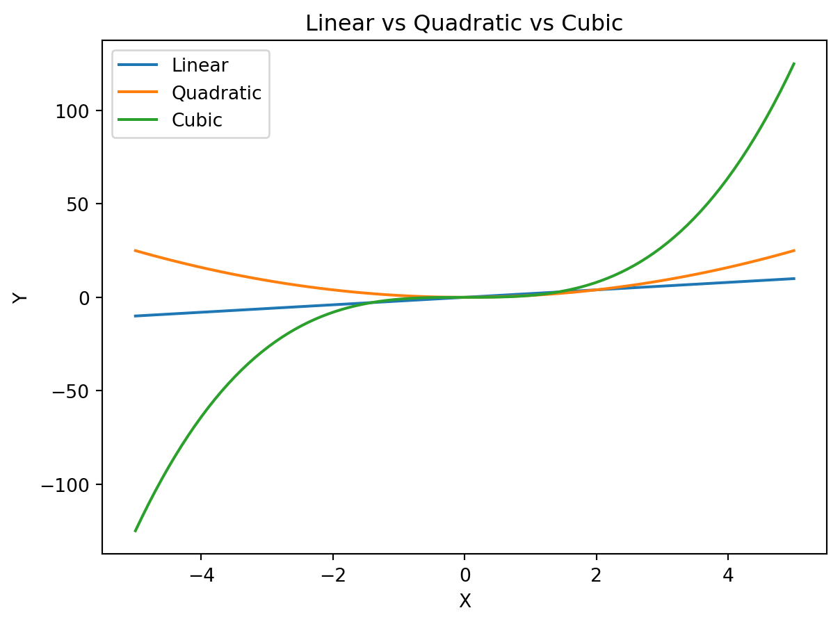
2C.3 Visualizing Polynomial Shapes

2C.4 Simulating a Curved Relationship (What We Are Doing and Why)

Before fitting models, we will create data where we know the true relationship is curved.

This is important for teaching because: - we control the true relationship, - we can see when a model is right or wrong, - and we can connect diagnostics back to the truth.

What this means

The true relationship is not linear
It increases at first, then bends downward
The noise term adds randomness (like real data)

So: > A linear model will be wrong, and a quadratic model should do better

2C.5 Fitting a Linear Model vs a Polynomial Model

Now we fit two models:

Model 1: Linear (incorrect form)

This model assumes: - the relationship is a straight line

Model 2: Quadratic (closer to truth)

This model allows: - curvature - a turning point

Key idea

We are comparing: - a model that is too simple - versus a model that better matches the true structure

2C.6 Comparing the Fits and Residuals

Step 1: Compare the fitted lines

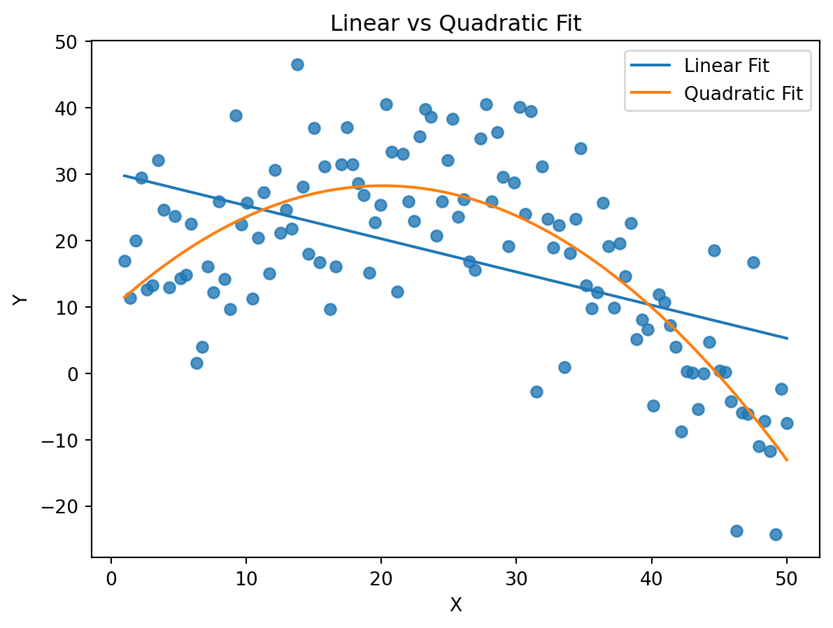
Interpretation

The linear model tries to force a straight line through curved data
The quadratic model follows the shape of the data more closely

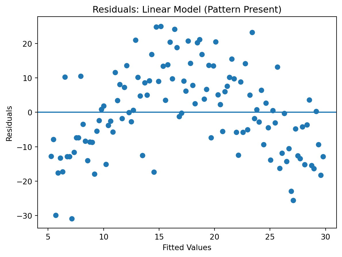
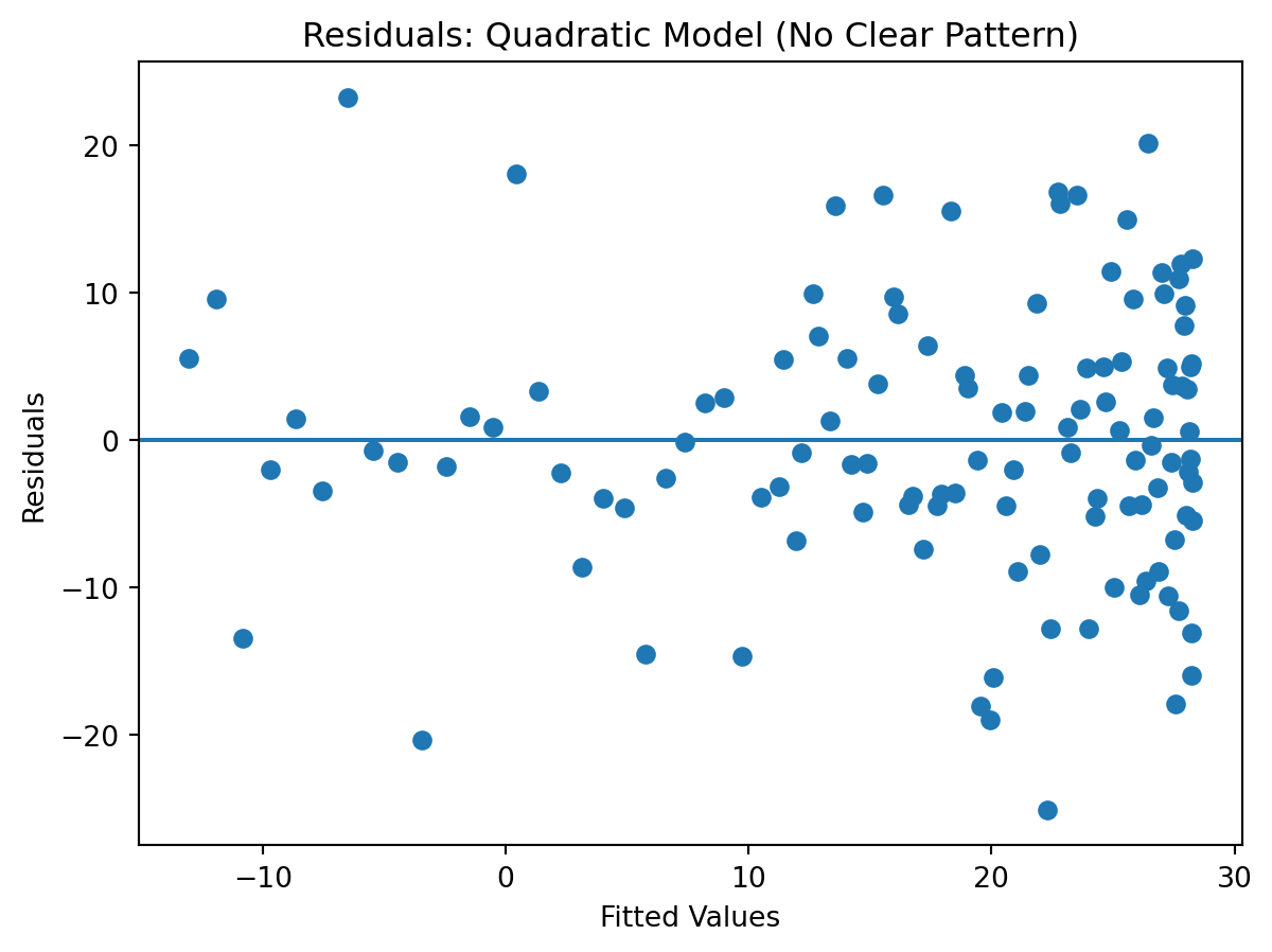
Step 2: Compare residuals

Critical interpretation (this is the key teaching point)

Linear model residuals

You will see a clear curved pattern
This means:
- the model is systematically wrong
- it is missing structure
- it violates the linearity assumption

Quadratic model residuals

Residuals look more like a random cloud around zero
This means:
- the model is capturing the structure
- no obvious pattern remains
- the model is now more consistent with regression assumptions

Big takeaway

Polynomial regression is not just about improving fit visually.

It is about:

removing structure from residuals
making the model consistent with regression assumptions
improving interpretation and reliability

2C.7 Significance of Polynomial Terms

Each term has its own hypothesis test:

\[ H_0: \beta_k = 0 \]

Key rule

When you are deciding whether to keep a polynomial form, focus on the highest-order term currently in the model.

For example:

in a quadratic model, focus on the p-value for \(X^2\)
in a cubic model, focus on the p-value for \(X^3\)

If the highest-order term is significant, that suggests the added curvature matters.

If the highest-order term is not significant, that is evidence that the more complex version may not be needed.

Important caution

This does not mean the lower-order terms are unimportant conceptually. It means the decision about whether you need the added complexity is driven by the highest-order term.

2C.8 Hierarchical Model Principle

Polynomial regression is hierarchical.

If you include: - \(X^3\)

you should also include: - \(X\) - \(X^2\)

Even if the lower-order terms are not individually significant.

Why?

Because: - higher-order terms build on lower-order structure - dropping lower terms usually makes the model harder to interpret - the polynomial is meant to be treated as a connected shape, not as unrelated separate pieces

Practical rule

Keep the lower-order terms whenever a higher-order term is included.

2C.9 Centering Variables (Important in JMP)

JMP often centers \(X\) before creating polynomial terms.

That means it creates:

\[ X_{centered} = X - \bar{X} \]

and then forms: - \(X_{centered}^2\) - \(X_{centered}^3\)

Why centering helps

Centering can:

reduce multicollinearity among polynomial terms
make coefficients more numerically stable
make the lower-order coefficients easier to interpret Note: this is a hold over from old beliefs, but does not change fit. It is just the way its implemented in JMP.

Very important point

Centering does not change:

fitted values
predicted values
overall model fit
residuals
which model is best

It only changes:

how the coefficients are expressed

So if JMP centers the variable, the curve itself does not change. Only the coefficient representation changes.

2C.10 Example Output

print(model_quad.summary())

                            OLS Regression Results                            
==============================================================================
Dep. Variable:                      y   R-squared:                       0.591
Model:                            OLS   Adj. R-squared:                  0.584
Method:                 Least Squares   F-statistic:                     84.64
Date:                Tue, 07 Apr 2026   Prob (F-statistic):           1.85e-23
Time:                        16:03:41   Log-Likelihood:                -436.06
No. Observations:                 120   AIC:                             878.1
Df Residuals:                     117   BIC:                             886.5
Df Model:                           2                                         
Covariance Type:            nonrobust                                         
==============================================================================
                 coef    std err          t      P>|t|      [0.025      0.975]
------------------------------------------------------------------------------
const          9.6425      2.708      3.561      0.001       4.279      15.006
x              1.8547      0.245      7.580      0.000       1.370       2.339
x2            -0.0462      0.005     -9.919      0.000      -0.055      -0.037
==============================================================================
Omnibus:                        0.126   Durbin-Watson:                   2.006
Prob(Omnibus):                  0.939   Jarque-Bera (JB):                0.024
Skew:                          -0.034   Prob(JB):                        0.988
Kurtosis:                       3.008   Cond. No.                     3.65e+03
==============================================================================

Notes:
[1] Standard Errors assume that the covariance matrix of the errors is correctly specified.
[2] The condition number is large, 3.65e+03. This might indicate that there are
strong multicollinearity or other numerical problems.

What to look for

Is \(X^2\) significant?
Does the quadratic shape improve fit?
Do residuals improve?

2C.11 Overfitting Example (High Order Polynomial)

Below is a much higher-order model on a small noisy dataset.

This is the kind of situation where a model can start fitting random variation instead of real structure.

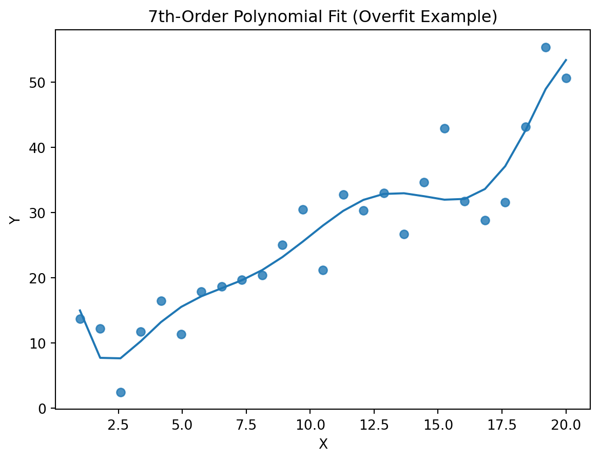
What students should notice

The curve can wiggle sharply
The shape may not make business sense
The model may be fitting noise, not signal

2C.12 Practical Guidance on Polynomial Order

Warning

In most practical business settings, it is wise to stay in the:

\(X^2\) range (quadratic)
or sometimes \(X^3\) range (cubic)

Only go higher if there is a strong theoretical reason or a very clear business reason to do so.

The higher the order: - the more flexible the model, - the greater the risk of overfitting, - and the harder the model becomes to explain.

2C.13 Why Overfitting Is Dangerous

Overfitting can lead to:

misleading significance
unstable coefficients
poor predictions on new data
curves that look impressive but are not trustworthy

That is why:

a more flexible model is not automatically a better model

2C.14 How to Evaluate Polynomial Models

Students should ask:

Did residuals improve in a meaningful way?
Is the highest-order term significant?
Does the overall curve make business sense?
Is the model stable, or is it chasing noise?
Is the extra complexity worth it?

2C.15 Practical Interpretation Example

\[ \hat{Y} = 10 + 3X - 0.1X^2 \]

Interpretation:

At lower values of \(X\), \(Y\) increases as \(X\) increases
At higher values of \(X\), the negative \(X^2\) term begins to pull the curve downward
This is a common way to represent diminishing returns

2C.16 JMP Workflow

Go to Analyze → Fit Model
Add the original \(X\) term
Add polynomial terms such as \(X^2\) or \(X^3\)
Review:
- the p-value for the highest-order term
- residual plots
- whether the curve makes business sense

If JMP uses centered polynomial terms, remember:

the fitted curve is the same
only the coefficient representation changes

2C.17 Common Mistakes

Using very high-order polynomials automatically
Ignoring the hierarchical structure
Dropping lower-order terms just because they are not significant
Looking only at significance and ignoring shape
Ignoring residual plots
Treating a wiggly curve as evidence of insight

2C.18 Check Your Understanding

Why would we use polynomial regression instead of a straight line?
In a quadratic model, which term’s p-value is most important for deciding whether curvature matters?
Why do we keep lower-order terms in the model even if they are not individually significant?
What does centering do in JMP when fitting polynomial models?
Does centering change the actual fitted curve?
Why are very high-order polynomials risky?

2C.19 Key Takeaways

What to remember from Part 2C

Polynomial regression captures curved relationships
The highest-order term is the key test for whether added curvature matters
Polynomial models should be treated as hierarchical
Lower-order terms stay in the model when higher-order terms are included
Centering improves numerical stability but does not change the fitted curve
Very high-order polynomials are risky and should usually be avoided unless strongly justified
Residual plots remain one of the best ways to judge whether the polynomial model is actually improving the fit